Gradient Descent Application - Reinforcement Learning
Introduction
In this tutorial, you will learn how to use OpenAI gym to create a controller for the classic pole balancing problem, and test what you learned on a rocket landing problem. Both will be solved using Reinforcement Learning. While fully understanding RL would require background knowledge beyond what we have covered in this class (namely, Markov Decision Process, Dynamic Programming, and Policy Search), here we present one particular formulation of an optimization problem for designing a controller, and show that gradient descent can be applied to solve this problem.
It should be noted that a controller for pole balancing can be designed and analyzed through classic control theory, by linearizing its dynamics. The presented solution here does not require knowledge about the dynamical system, nor does it require linearization (is it good news or not?).
Get Ready
This section discusses the preparation you need to kick start the project. We will start with a minimalistic guideline, and then introduce all gadgets involved (Git, Github, Python, and TensorFlow) for those who are interested.
A minimalistic guideline to get things to work (without Docker)
This guideline is written for Windows users and tested on Windows only. For Linux and Mac users, you can follow the guideline, although you should already have Python and Git installed by default.
-
To download the cartpole sample code, you can either click on the green button (Clone or download) to download as a zip, or use Git(See intro to Git).
-
You will install Python 3.5. Check if Python is correctly installed by typing in the command line
python. To do so, launch the command prompt (go to start and searchcmd). IMPORTANT: When you install Python, please choose to install pip, and choose to include Python in your environment path. -
Install TensorFlow (CPU version) here if you are on Linux or Mac, or here if you are on Windows.
-
Once done, go to the folder where you hold this code, type in the command line:
pip install -r requirement.txt. This should install all dependencies. IMPORTANT: Please run this command in the command line, rather than in the Python prompt. -
You can then run the code by typing in:
python main.py.
A little more details on the gadgets involved
The following would be useful if you plan to build your course project using Python, TensorFlow, or Github.
-
Development Environment: I recommend Pycharm. This is an environment where you can manage all Python versions, packages, and version control, which I will explain next. NOTE: As a student, you can get a free license for Pycharm.
-
Version control: The idea of version control is to keep track of all changes you make throughout the project so that you can always trace back to an earlier version of your project. It also make collaboration more seamless, e.g., by automatically merging together different versions of the same document produced by members of a team. Git is arguably the most popular version control package out there right now. Once you install git, you can ask it to track any document you work on, e.g., texts, codes, etc. Here we use git to both clone an existing project from github, and to version control that cloned project locally.
-
Github: Github is the place where your store your project for free, as long as the project is made publicly available. It is becoming a standard in academia and some industry that codes and data be published on github so that results claimed by researchers can be reproduced. In this class, you are required to publish your project on github so that your models can be reused by future students (depending on your choice of the license), and your results can be reproduced if necessary.
Pole balancing
If you successfully get the example code to run, and wonder what happened under the hood, please read on.
Problem statement
The simple pole balancing (inverse pendulum) setting consists of a pole and a cart. The system states are the cart displacement \(x\), cart velocity \(\dot{x}\), pole angle \(\theta\), and pole angular velocity \(\dot{\theta}\). The parameters of the default system is as follows:
| Left-aligned | Center-aligned |
|---|---|
| mass cart | 1.0 |
| mass pole | 0.1 |
| pole length | 0.5 |
| force | 10.0 |
| delta_t | 0.02 |
| theta_threshold | 12 (degrees) |
| delta_t | 2.4 |
The controller takes in the system states, and outputs a fixed force on the cart to either left or right. The controller needs to be designed so that within 4 seconds, the pole angle does not exceed 12 degrees, and the cart displacement does not exceed 2.4 unit length. A trial will be terminated if the system is balanced for more than 4 seconds, or any of the constraints are violated.
Some preliminaries for reinforcement learning
We first introduce the concept of a Markov Decision Process: An MDP contains a state space, an action space, a transition function, a reward function, and a decay parameter \(\gamma\). In our case, the state space contains all possible combinations of \(x\), \(\dot{x}\), \(\theta\), \(\dot{\theta}\). The action space contains the force to the left, and the force to the right. The transition function \(s_{k+1} = T(s_k,a_k)\) computes the next state \(s_{k+1}\) based on the current state \(s_k\) and the action \(a_k\).
The transition is given by the system equations. The reward function defines an instantaneous reward \(r_k = r(s_k)\). In particular, we define reward as 1 when the system does not fail, or 0 otherwise. A discount factor \(\gamma\) is applied to rewards so that rewards in the far future worth less than the near future. A long term value function is defined recursively as a function of the controller \(\pi\):
\[V_k(\pi,s_k) = r_k + \gamma V_{k+1}(\pi,T(s_k,a_k)).\]We define the controller as a function of the states that outputs a number between 0 and 1: \(\pi(s,w) \in [0,1]\), where \(w\) is the unknown parameters to be learned. This number will be treated as the probability for choosing the action “pushing to the left”. The probability for “pushing to the right” will be \(1-\pi(s,w)\).
Due to the randomness in the initial state \(s_0\) and the sequence of actions \(a_0\), \(a_1\),…, \(a_K\), the value function \(V_0(\pi,s_0)\) is a random variable parameterized by \(w\).
The goal of optimal control is to find optimal controller parameters \(w\) that maximizes the expectation of the value
\[\mathbb{E}_{s_0,a_0,a_1,...,a_K}[V_0(\pi,s_0)].\]A simple loss function
Given a trial run with \(K\) time steps based on the current controller, we collect the instantaneous rewards \(r_k\), actions \(a_k\), and the controller outputs \(\pi_k\) for \(k=1,...,K\). We can minimize the following loss function
\(f(w) = -\sum_{k=1}^K (\sum_{j=k}^K \gamma^{j-k}r_j) (a_k\log(\pi_k)+(1-a_k)\log(1-\pi_k))\).
In this loss function, the first term \(\sum_{j=k}^K \gamma^{j-k}r_j\) represents the value at time step \(k\), the second term \(a_k\log(\pi_k)+(1-a_k)\log(1-\pi_k)\) is close to \(0\) when the favored action is chosen, and \(-\inf\) when the unfavored action is chosen. Essentially, the loss is minimized when all chosen control decisions \(a_k\) lead to high value. Thus by tuning \(w\), we correct the mistakes we made in the trial (i.e., high value from unfavored move, or low value from favored move).
In the code, you may notice that the values are normalized. According to this paper, this treatment speeds up the training process.
Controller model
We mentioned that the controller computes a probability \(\pi(s,w)\). But how does this function look like? Here we model \(\pi(s,w)\) as a single-layer neural network:
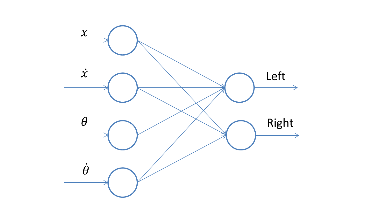
It is found that a single layer is sufficient for this environment setting. In fact, adding layers may deteriorate the training performance due to the additional network complexity.
Training algorithm
Due to the probabilistic nature of the controller, we minimize an averaged loss \(\bar{f}(w) = \sum_{t=1}^T f_t(w)\) over \(T\) trials. This is done by simply running the simulation \(T\) times, recording all data, and calculate the gradient of \(\bar{f}(w)\). Notice that the gradient in this case will be stochastic, in the sense that we only use \(T\) random samples to approximate it, rather than finding the theoretical mean of \(\nabla_w \bar{f}\). We use [ADAM][adam] to perform stochastic gradient descent.
Results
With default problem settings, we can get a convergence curve similar this:
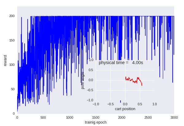
Y axis of the main plot is the total reward a policy achieves, X axis is the number of training epochs. The small window shows the normalized trajectory of cart positions and pole angles in the most recent trial. It can be seen that the learning achieves a good controller in the end.
To store videos, you will need to uncomment the line:
# self.env = wrappers.Monitor(self.env, dir, force=True, video_callable=self.video_callable)
By doing this, a series of the simulation videos will be saved in the folder /tmp/trial.
You can change problem parameters in gym_installation_dir/envs/classic_control/cartpole.py.
More details about the setup of this physical environment can be found
in the gym documents.
Details on how to derive the governing equations for single pole can be
found at this technical report.
Corresponding equations for how to generalize this to multiple poles
can also be found at this paper
Rocket landing
The rocket landing case is created by my former student Steven Elliott. The report is here. Below is a brief introduction to his code.
Problem statement
The rocket has 6 states: the x and y coordinates, the angle, and the time derivative of these three. The action space is discrete:
- Action 0 - No thrust, no torque
- Action 1 - No thrust, torque left
- Action 2 - No thrust, torque right
- Action 3 - Trust, no torque
- Action 4 - Thrust, torque left
- Action 5 - Thrust, torque right
The reward is defined as the negative of the Euclidean distance from the last position of the rocket to the target landing location.
Exercise
Please test the code and think about the following questions.
-
What do you think is a good objective function to use for the training?
-
How will you formulate the problem if the dynamics of the rocket is known?