From Finite Element Analysis to Topology Optimization
This note introduces the basic concept of finite element analysis (FEA) and topology optimization (Topopt), and hopefully convince you that these are important topics to learn about for future engineers and entrepreneurs.
The FEA examples are from this tutorial.
1D Finite Element Analysis
In the class we covered the deflection analysis for regular beams under various loads. The analysis of irregular beams and structures of other topologies will rely on finite element analysis (FEA).
FEA is an involving topic. Thus I will only cover the very basic ideas so that we can use them to introduce topology optimization.
A two-spring system
Consider the two element system where Node 1 is attached to a fixed support, yielding the displacement constraint \(U_1 = 0\), \(k_1= 50 lb/in\), \(k_2= 75 lb/in\), \(F_2=F_3= 75 lb\). For these conditions determine nodal displacements \(U_2\) and \(U_3\).
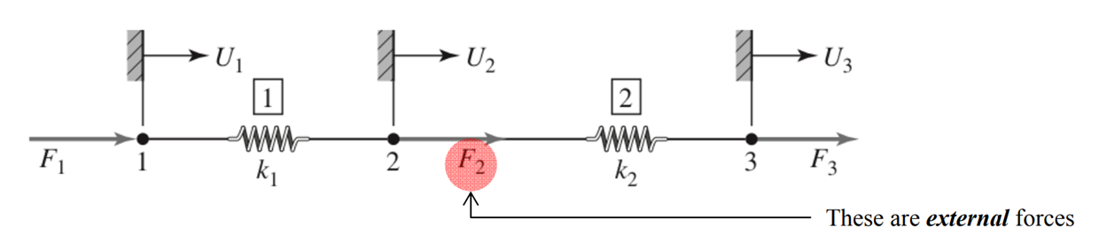
The displacements satisfy the following equation:
\[\begin{bmatrix} 50&-50&0\\-50&125&-75\\0&-75&75 \end{bmatrix} \begin{bmatrix} 0\\U_2\\U_3 \end{bmatrix} =\begin{bmatrix} F_1\\75\\75 \end{bmatrix}\]Solve this to have \(U_2=3\) and \(U_3=4\). This is a simplest example of FEA, where the two springs represent the elements, the ends of the springs the nodes. The matrix \({\bf K}=\begin{bmatrix} 50&-50&0\\-50&125&-75\\0&-75&75 \end{bmatrix}\) is the global stiffness matrix, and \({\bf U} = \begin{bmatrix} 0\\U_2\\U_3 \end{bmatrix}\) the global displacement vector.
Truss element example
Now consider a tapered elastic bar subjected to an applied tensile load \(P\) at one end and attached to a fixed support at the other end. The cross-sectional area varies linearly from \(A_0\) at the fixed support at \(x = 0\) to \(A_0/2\) at \(x = L\). Calculate the displacement of the end of the bar (a) by modeling the bar as a single element having cross-sectional area equal to the area of the actual bar at its midpoint along the length, (b) using two bar elements of equal length and similarly evaluating the area at the midpoint of each, and compare to the exact solution.
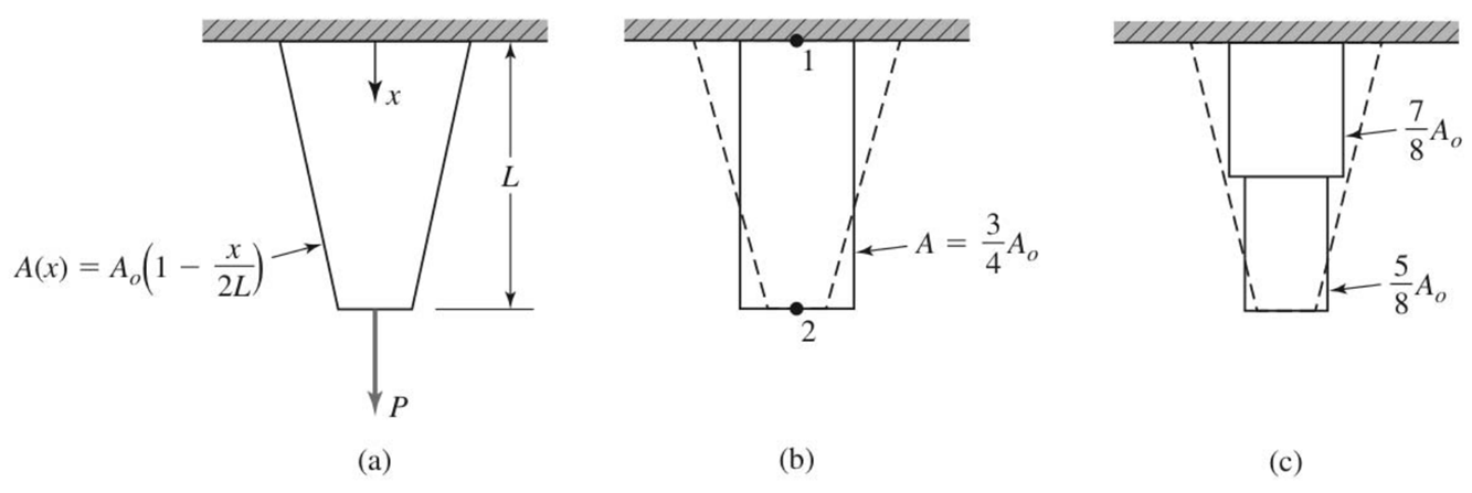
We know that the equivalent stiffness of each element is \(k = P/\delta = AE/L\) (the strain \(\delta = PL/AE\)).
(a) \(k=AE/L=3A_0E/4L\) and \(3A_0E/4L \begin{bmatrix} 1&-1\\-1&1 \end{bmatrix} \begin{bmatrix} U_2\\U_3 \end{bmatrix} = \begin{bmatrix} F_1\\P \end{bmatrix}\). This leads to \(U_2 = 1.33PL/A_0E\)
(b) Two elements of equal length \(L/2\) with associated nodal displacements. For element 1, \(A1 = 7A_0/8\) so \(k_1 = 7A_0E/4L\), while for element 2, \(A_1 = 5A_0/8\) and \(k_2 = 5A_0E/4L\).
From \(\begin{bmatrix} k_1&-k_1&0\\-k_1&k_1+k_2&-k_2\\0&-k_2&k_2 \end{bmatrix} \begin{bmatrix} U_1\\U_2\\U_3 \end{bmatrix} =\begin{bmatrix} F_1\\0\\P \end{bmatrix}\) and \(U_1 = 0\) we get \(U_2 = 4PL/7A_0E\) and \(U_3 = 1.371 PL/A_0E\).
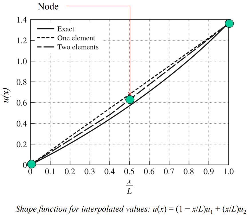
The exact solution is 1.386PL/A_0E. With two elements, we have a better approximation of the solution. Including more elements will further improve the approximation.
Topology Optimization
We showed that the deflection or deformation of a structure (\({\bf U}\)) can be solved through a algebraic equation
\({\bf KU}={\bf F}\).
It can be further shown that the strain energy due to the deformation is \(0.5{\bf U}^T{\bf KU}\). Minimizing this energy is equivalent to minimizing the compliance of the structure under the given loads and boundary conditions, leading to optimal topologies.
We explain some technical details below. A good tutorial can be found from Dr. Sigmund’s group (see e.g., this code and this paper).
The compliance minimization problem
Topology optimization has been commonly used to design structures and materials with optimal mechanical, thermal, electromagnetic, acoustical, or other properties. The structure under design is segmented into \(n\) finite elements, and a density value \(x_i\) is assigned to each element \(i \in \{1,2,...,n\}\): A higher density corresponds to a less porous material element and higher Yong’s modulus. Reducing the density to zero is equivalent to creating a hole in the structure. Thus, the set of densities \({\bf x}=\{x_i\}\) can be used to represent the topology of the structure and is considered as the variables to be optimized. A common topology optimization problem is compliance minimization, where we seek the “stiffest” structure within a certain volume limit to withhold a particular load:
\[\min_{\bf x} \quad {\bf f} := {\bf U}^T {\bf K}({\bf x}) {\bf U}\] \[\text{subject to:} \quad {\bf h} := {\bf K}({\bf x}) {\bf U} = {\bf F},\] \[\quad {\bf g} := V(\textbf{x}) \leq v,\] \[\textbf{x} \in [0,1].\]Here \(V(\textbf{x})\) is the total volume; \(v\) is an upper bound on volume; \({\bf U} \in \mathbb{R}^{n_d\times 1}\) is the displacement of the structure under the load \({\bf F}\), where \(n_d\) is the degrees of freedom (DOF) of the system (i.e., the number of x- and y-coordinates of nodes from the finite element model of the structure); \({\bf K(x)}\) is the global stiffness matrix for the structure.
\({\bf K(x)}\) is indirectly influenced by the topology \({\bf x}\), through the element-wise stiffness matrix
\({\bf K}_i = \bar{\bf K}_e E(x_i)\),
where the matrix \(\bar{\bf K}_e\) is predefined according to the finite element type and the nodal displacements of the element, \(E(x_i)\) is the element-wise Young’s modulus defined as a function of the density \(x_i\): \(E(x_i) := \Delta E x_i^p + E_{\text{min}}\), where \(p\) (the penalty parameter) is usually set to 3. This cubic relationship between the topology and the modulus is determined by the material constitutive models, and numerically, it also helps binarize the topologies, i.e., to push the optimal \({\bf x}_i\) to 1 or 0 (why?). The term \(E_{\text{min}}\) is added to provide numerical stability.
For those interested, here I explain the details for solving this topology optimization problem.
Application of Topology Optimization
While the theories behind topology optimization were developed during the 1980s, the value of this technique only started to show after manufacturing and in particular 3D printing technologies become more matured in the last two decades. Today topology optimization has many industry applications, from light-weight vehicle bodies, to artificial bones and implants, to biomemetic airplane wings, to various sensors and actuators.
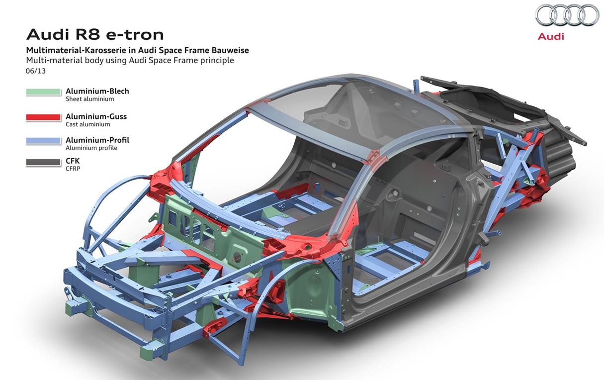
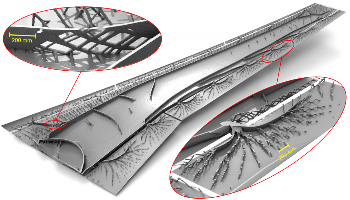
Image from Aage et al. (2017) “Giga-voxel computational morphogenesis for structural design”
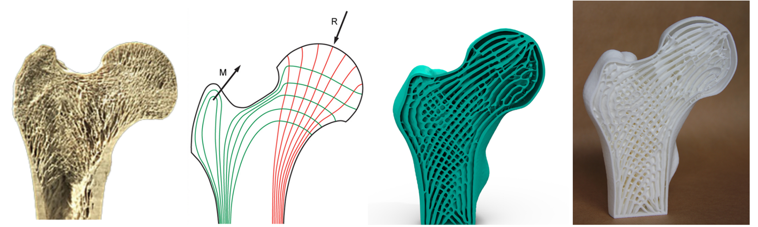
Image from Wu et al. (2018) “Infill Optimization for Additive Manufacturing - Approaching Bone-like Porous Structures”
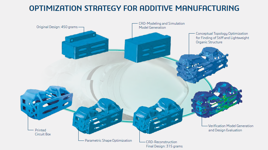
Image from Dassault Systems