A Tutorial on Curve Fitting

As you have seen through the class, curve fitting happens all the time through the development of engineering knowledge, due to the fact that we often have the ability to observe things before we understand them. Thus curve fitting almost always indicate a sub-optimal solution due to the lack of more rigorous methodology or time. But since engineering design is so complicated, it becomes a regular part of engineers’ thinking.

In this tutorial, I will first go through the very basic techniques of curve fitting, which you may have already learned through Excel or Matlab. I will then talk about more broadly the issue of curve fitting. The purpose is for you to understand that when people talk about machine learning and AI, they are often talking about “curve fitting”.

You may also want to check my slides on this topic and the enormous amount of tutorials online. The fancy keywords are “regression”, “supervised learning”, “meta-modeling”.

Let’s define “curve fitting”

Curve fitting, or formally supervised learning, deals with labeled data \(\mathcal{D} = [{\bf x}_1,{\bf y}_1,{\bf x}_2,{\bf y}_2,\cdots]\) where \({\bf x}\) is the input and \({\bf y}\) the output (or the label). For example, the inputs can be Trump’s tweets and the outputs the stock market performance right after that; or the inputs material microstructures and the outputs their fracture strength; or the inputs camera images and the outputs recognitions of objects within the images; or the inputs graphical representations of chemical compounds and the outputs the survival rate of test specimens; or …this can go on forever.

In its simplest setting, supervised learning deals with scalar or vectorial inputs and scalar outputs. The goal is to fit a curve (for 1D input) or a surface (for 2D input) or a hypersurface (for nD input) to the data so that when a new input is given, we can find an accurate prediction of the corresponding output from the curve or surface or hypersurface. Often the question is: Do I use a straight line to fit or some kind of curve? How do I decide? An important concept to learn here is the Occam’s razor. To put this into context, the prediction accuracy of your curve goes up when the curve fit well with the data, but also goes down if your curve is too wavy. In other words, you want to find a curve (e.g., a polynomial function of a certain degree) that fits through most of the data points (no under-fitting) but do not overfit. Common approaches to this include information criteria (check AIC and BIC) and cross-validation.

How do you do curve fitting in Matlab?

Let’s now talk about how to actually do curve fitting without going deeper into the theory.

Curve fitting with scalar input

In Matlab, this can be done using the polyfit() function when the input is scalar. Required inputs are the sampled input and output data, and the degree of the desired polynomial. The output is a \(n+1\) length vector describing the polynomial coefficients where \(n\) is the degree of the polynomial.

After finding the polynomial coefficients, its easiest to use the polyval() function to evaluate the polynomial at the desired \({\bf x}\) values. This can be more explicitly represented as: y = p(1).*x.^n + p(2).*x.^(n-1) + ... + p(n).*x + p(n+1).

An example in use is below along with visualization of over-fitting and under-fitting:

x = [0.0426 0.1210 0.1555 0.2661 0.3629 0.4551 0.5703 0.6924 0.7846 0.8583];
y = [0.1006 0.2464 0.3834 0.5525 0.7274 0.7070 0.5671 0.5816 0.5525 0.5962];

p = polyfit(x,y,degree);

x_fit = 0:0.01:1;
y_fit = polyval(p,x_fit);

figure; hold on;
plot(x,y,'o')
plot(x_fit,y_fit)

Under-fit

Good-fit

Over-fit

Curve fitting with vectorial input

Often times your inputs are vectors (e.g., images, structures, texts, audios, etc.). The Matlab curve fitting toolbox has a whole bunch of tools for fitting vectorial inputs to scalar (or vectorial) outputs. If the toolbox is not free to you, I highly recommend sk-learn as a free and better alternative. Sk-learn is very well documented and has plenty of examples for you to follow.

Without going too much into the software details, I want to summarize a few important categories of curve fitting models that are often used in engineering, with their pros and cons. You will need to find their implementations either from Matlab, or sk-learn, or other places.

• Linear models: These are the most widely used and are often very effective. Note that linear here does not mean that the model can only fit straight lines. In fact, this category includes all polynomial curves and beyond (as long as the model is linear in the parameter space). Pros: Easy to use. Implementation can be found everywhere (start with Matlab). Cons: Don’t work well when the data is too wavy. You will need to define how the curve look like (e.g., the degree of a polynomial function).

• Kernel machines: A typical kernel machine is the Support Vector Machine (SVM). I will skip the technical details since SVM has been a standard and you can find tutorials on it easily. To summarize, SVM with nonlinear kernel is non-parametric, meaning that they can fit through all data points using the smoothest curve if needed and can automatically prevent overfitting through hyperparameter tuning. Yes, that’s a lot, but everything is automated in standard SVM packages, e.g., libSVM (also included in sk-learn) and Matlab’s fitrsvm. Pros: Very flexible. Can handle complicated input-output relations and high-dimensional inputs. Cons: Curve fitting takes longer (in general scales with the square of the number of data points) and takes more storage space. Model not interpretable.

• Gaussian process: Similar to SVM with nonlinear kernel, GPs are non-parametric and can fit through all data points perfectly. Thus GP is commonly used to fit simulation data (where no measurement noise is assumed). Pros: Very flexible. Can handle complicated input-output relations. The model naturally provides uncertainty of the prediction. Cons: Curve fitting takes longer (in general scales with the square of the number of data points) and takes more storage space. Accuracy of the model is sensitive to hyperparameter tuning.

• Neural network: This is probably the most popular tool for curve fitting with all the successful applications of deep learning. Unlike kernal machines and Gaussian process though, we still don’t have much theory developed to guide the construction of neural networks, and we only know they work when they actually work! Pros: Somehow, they often work when you have a lot of data and know all the tricks in training them. Cons: Even when you believe they work, you don’t know when they don’t.

From curve fitting to real engineering challenges

There are several reasons why curve fitting is a good idea for solving engineering problems (while not necessarily the best idea). I will summarize with the following:

• Accelerate computation: We have shifted most of the engineering practices from experiments to simulations to speed up the design and validation processes. However, engineering simulations are still very slow, especially when dealing with complex systems and when fidelity matters. For example, vehicle crash, material fatigue, and CFD simulations still takes hours on high-performance computers. Curve fitting can potentially accelerate such simulations, i.e., we can build predictive models based on previous simulation data to circumvent future call of expensive simulations. See this video on an accelerated Navier-Stokes solver for example. The same technique can be applied to accelerate a large range of engineering simulations.

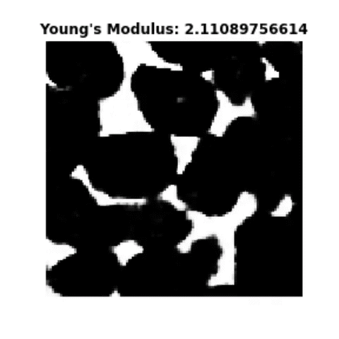
• Accelerated design: One benefit of accelerating simulations is that now we can evaluate (and thus optimize) new engineering designs faster. See for example the following process where we optimize a material microstructure towards higher or lower Young’s modulus based on a “curve” that predicts the modulus based on the microstructure.

What’s difficult?

I will end with a brief discussion on what is currently wrong with curve fitting, and particularly their applications to engineering domains. Overall, as we move from scenarios with simple data and simple models (e.g., linear models and kernel machines) to those with high-dimensional data and complex models (e.g., neural networks), we loose the capability to tell when things will go wrong. In fact, things are going wrong. For example, we now know that vision systems on autonomous cars can be attacked to recognize stop signs as speed limit signs (search adversial attack to see most recent developments in this direction). One can imaging that when we use complex “curves” to fit engineering data, things can also go wrong, i.e., an engineering design optimized by a machine based on a predictive model can be totally crap. The key issue is that our current knowledge about curve fitting does not lead to knowledge transfer of a machine, i.e., a machine cannot do extrapolation or even interpolation well with the data presented. See this lecture from Yann Lecun on this broadly existing issue.