Tutorial on Topology Optimization

Compliance minimization with local density constraint (created by Ruijin Cang)
Introduction
With great power comes great responsibility. The recent advances in 3D printing (overview slides) allowed unprecedented opportunities in creating complex geometries for all kinds of applications from soft robots to customized prosthetics to light-weight energy absorbers. The question is: How do we systematically create these complex geometries? Topology optimization is the answer.
The goal of this tutorial is to help you to learn topology optimization without any background knowledge, although you do need to be prepared for calculus and linear algebra. Please also read my previous post on finite element analysis if you are not familiar with the topic.
The tutorial is modified from my post for the optimization class, with additional explanations added when necessary. It is also based on Dr. Sigmund’s topology optimization code and paper.
Explanation of the mathematical problem behind compliance minimization
Recall that one typical form of topology optimization uses the compliance of the structure as the design objective. Two reasons for this: One, it is common that one wants a structure to be compliant or stiff (or a mixture of both); second, compliance is not only easy to compute but also (relatively) easy to differentiate, which, as we will see, is the key to topology optimization.
Notations
Following the previous discussion, the structure under design is segmented into \(n\) finite elements, and a density value \(x_i\) is assigned to each element \(i \in \{1,2,...,n\}\): A higher density corresponds to a less porous material element and higher Yong’s modulus. Reducing the density to zero is equivalent to creating a hole in the structure. Thus, the set of densities \({\bf x}=\{x_i\}\) can be used to represent the topology of the structure and is considered as the variables to be optimized. See figure here.
Problem statement
The compliance minimization problem is formulated as follows:
\[\min_{\bf x} \quad {\bf f} := {\bf d}^T {\bf K}({\bf x}) {\bf d}\] \[\text{subject to:} \quad {\bf h} := {\bf K}({\bf x}) {\bf d} = {\bf u},\] \[\quad {\bf g} := V(\textbf{x}) \leq v,\] \[\textbf{x} \in [0,1].\]Here \(V(\textbf{x})\) is the total volume; \(v\) is an upper bound on volume; \({\bf d} \in \mathbb{R}^{n_d\times 1}\) is the displacement of the structure under the load \({\bf u}\), where \(n_d\) is the degrees of freedom (DOF) of the system (i.e., the number of x- and y-coordinates of nodes from the finite element model of the structure); \({\bf K(x)}\) is the global stiffness matrix for the structure.
\({\bf K(x)}\) is indirectly influenced by the topology \({\bf x}\), through the element-wise stiffness matrix
\[{\bf K}_i = \bar{\bf K}_e E(x_i),\]and the local-to-global assembly:
\[{\bf K(x)} = {\bf G}[{\bf K}_1,{\bf K}_2,...,{\bf K}_n],\]where the matrix \(\bar{\bf K}_e\) is predefined according to the finite element type (we use first-order quadrilateral elements throughout this tutorial) and the nodal displacements of the element (we use square elements with unit lengths throughout this tutorial), \({\bf G}\) is an assembly matrix, \(E(x_i)\) is the element-wise Young’s modulus defined as a function of the density \(x_i\): \(E(x_i) := \Delta E x_i^p + E_{\text{min}}\), where \(p\) (the penalty parameter) is usually set to 3. This cubic relationship between the topology and the modulus is determined by the material constitutive models, and numerically, it also helps binarize the topologies, i.e., to push the optimal \({\bf x}_i\) to 1 or 0 (why?). The term \(E_{\text{min}}\) is added to provide numerical stability.
Design sensitivity analysis
Design sensitivity analysis is about computing the gradient \(\frac{df}{d{\bf x}}\), i.e., the sensitivity of the objective (compliance) with respect to the changes in the topology. This gradient represents the direction of unit topological change that will increase the compliance the most (or decrease the most if the negative gradient direction is taken). Therefore, once the gradient is derived, one can simply apply gradient ascend (or descend) to maximize (or minimize) the compliance. Analogously, knowing the gradient is the same as knowing which way to climb up (or down) the mountain.
By knowing this, one can see that design sensitivity analysis is key to all optimization problems. However, for topology optimization and many other problems, deriving the sensitivity (the gradient) is often not straight forward or in some cases very challenging. We will explain in the following why this is so and how the derivation is done in our specific case.
In general, the challenge comes from the fact that the objective \(f\) (the function we are trying to optimize) is a function of the states, which are not explicitly known without solving some governing equations. In our case, the states are the displacements \({\bf d}\) and variables are the density values \({\bf x}\). We also notice that states and variables are related through the equation \({\bf h} := {\bf K}({\bf x}) {\bf d} = {\bf u}\), which means that the states are implicitly functions of the variables. Therefore, the sensitivity \(\frac{df}{d{\bf x}}\) can be calculated as
\[\frac{df}{d{\bf x}} = (2 {\bf K}{\bf d})^T \frac{d{\bf d}}{d{\bf x}} + {\bf d}^T \frac{d{\bf K}}{d{\bf x}}{\bf d}\]The above equation requires the derivation of \(\frac{d{\bf d}}{d{\bf x}}\), which can be found by differentiating the equation \({\bf h}\):
\[\frac{d{\bf h}}{d{\bf x}} = \frac{d{\bf K}}{d{\bf x}}{\bf d} + {\bf K}\frac{d{\bf d}}{d{\bf x}} = {\bf 0}\]which leads to
\[\frac{d{\bf d}}{d{\bf x}} = {\bf K}^{-1}\frac{d{\bf K}}{d{\bf x}}{\bf d}\]Therefore
\[\frac{df}{d{\bf x}} = - {\bf d}^T \frac{d{\bf K}}{d{\bf x}}{\bf d}\]The above explains how the sensitivity is computed for our compliance minimization problem. It is worth noting that the result is only valid for (1) linear elastic material and (2) small deformation, under which the stiffness matrix \({\bf K}\) does not change during the bending of the structure and the governing equation is linear with respect to the states. In general, however, these assumptions do not hold and one will need to resort to adjoint method for computing the sensitivity. Please see this more involved but well written tutorial by Andrew Bradley.
The optimality conditions
In the above, we discussed about how to compute the design sensitivity for solving a topology optimization problem. We learned that the sensitivity (the gradient) can be treated as a force that “pushes” a current design to move towards better objective values. The question then is “when do we stop pushing?” Here is an intuitive answer: We stop when one of the two things happened: (1) when we reach a point where the force is zero; or (2) when we reach a point where there is a wall, so that the force and the “counter force” from the wall cancel out. Mathematically, the first case corresponds to a unconstrained solution (you learned this from calculus); the second case corresponds to a constrained solution, where constraints prevent us from further improving the solution.
Now consider compliance minimization. There are two kinds of constraints: One is that the density of the mesh can only go from 0 to 1; the other is that the total density (or volume) is constrained (through the volume fraction constraint). From the derived equation for sensitivity, one can see that this volume fraction constraint should always be active if an optimal topology is found, i.e., the optimal topology should have as much volume fraction as allowed (why?). From our intuitive understanding of the optimality conditions, this means that there will be a counter force from the wall through the volume fraction constraint.
This force balance, or the optimality conditions, can be expressed formally as
\[\frac{df}{d{\bf x}} + \mu \frac{d ({\bf 1}^T{\bf x}) }{d{\bf x}} = 0\]Here \({\bf 1}^T{\bf x}\) represents the total volume, thus \(\frac{d ({\bf 1}^T{\bf x}) }{d{\bf x}} = {\bf 1}\). \(-\frac{df}{d{\bf x}}\) pushes the solution towards lower compliance and \(- \mu {\bf 1}\) pushes towards lower volume. \(\mu \geq 0\) is called the Lagrangian multiplier, which measures the scale of the counter force, and is 0 when the solution does not “hit the wall”.
There are many ways to find solutions (in terms of \({\bf x}\) and \(\mu\)) to satisfy the optimality conditions. See for example the method of moving asymptotes (MMA) and augmented Lagrangian. One simple approach is to iteratively update \({\bf x}\) as
\[{\bf x}_{new} = \sqrt{-\frac{df}{d{\bf x}}/\mu}{\bf x}\]by choosing \(\mu\) in each iteration so that \({\bf x}_{new}\) is within 0 and 1. Note that the square root and the multiplication operations in the above equation are element-wise. The rationale is that from the optimality conditions, \(-\frac{df}{d{\bf x}}/\mu\) should converge to 1 at an optimal solution.
The algorithm
With these preliminaries, let us now look at the implementation. The seudo code for compliance minimization is as follows:
-
FEA setup (see details below)
-
Algorithm setup: \(\epsilon = 0.01\) (or any small positive number), \(k = 0\) (counter for the iteration), \(\Delta x =\) a number larger than \(\epsilon\)
-
While \(norm(\Delta x) \leq \epsilon\), Do:
3.1. Update the stiffness matrix \({\bf K}\) and the displacement (state) \({\bf u}\) (finite element analysis)
3.2. Calculate element-wise compliance \({\bf u}^T_i \bar{\bf K}_e {\bf u}_i\)
3.3. Calculate partial derivatives \(\frac{df}{dx_i} = - 3\Delta E x_i^2 {\bf u}^T_i \bar{\bf K}_e {\bf u}_i\)
3.4. The gradient with respect to the volume fraction constraint is a constant vector of ones (\([1,...,1]^T\))
3.5. Apply filter to \(\frac{df}{d{\bf x}}\) to smooth the gradient (See discussion below)
3.6. Update \({\bf x}\) as \({\bf x}_{new} = \sqrt{-\frac{df}{d{\bf x}}/\mu}{\bf x}\)
3.7. Update \(norm(\Delta x)\), \(k = k+1\)
Implementation details
We explain some details based on the classic 88 line topology optimization code.
The code
%%%% AN 88 LINE TOPOLOGY OPTIMIZATION CODE Nov, 2010 %%%%
function top88(nelx,nely,volfrac,penal,rmin,ft)
%% MATERIAL PROPERTIES
E0 = 1;
Emin = 1e-9;
nu = 0.3;
%% PREPARE FINITE ELEMENT ANALYSIS
A11 = [12  3 -6 -3;  3 12  3  0; -6  3 12 -3; -3  0 -3 12];
A12 = [-6 -3  0  3; -3 -6 -3 -6;  0 -3 -6  3;  3 -6  3 -6];
B11 = [-4  3 -2  9;  3 -4 -9  4; -2 -9 -4 -3;  9  4 -3 -4];
B12 = [ 2 -3  4 -9; -3  2  9 -2;  4  9  2  3; -9 -2  3  2];
KE = 1/(1-nu^2)/24*([A11 A12;A12' A11]+nu*[B11 B12;B12' B11]);
nodenrs = reshape(1:(1+nelx)*(1+nely),1+nely,1+nelx);
edofVec = reshape(2*nodenrs(1:end-1,1:end-1)+1,nelx*nely,1);
edofMat = repmat(edofVec,1,8)+repmat([0 1 2*nely+[2 3 0 1] -2 -1],nelx*nely,1);
iK = reshape(kron(edofMat,ones(8,1))',64*nelx*nely,1);
jK = reshape(kron(edofMat,ones(1,8))',64*nelx*nely,1);
% DEFINE LOADS AND SUPPORTS (HALF MBB-BEAM)
F = sparse(2,1,-1,2*(nely+1)*(nelx+1),1);
U = zeros(2*(nely+1)*(nelx+1),1);
fixeddofs = union([1:2:2*(nely+1)],[2*(nelx+1)*(nely+1)]);
alldofs = [1:2*(nely+1)*(nelx+1)];
freedofs = setdiff(alldofs,fixeddofs);
%% PREPARE FILTER
iH = ones(nelx*nely*(2*(ceil(rmin)-1)+1)^2,1);
jH = ones(size(iH));
sH = zeros(size(iH));
k = 0;
for i1 = 1:nelx
  for j1 = 1:nely
    e1 = (i1-1)*nely+j1;
    for i2 = max(i1-(ceil(rmin)-1),1):min(i1+(ceil(rmin)-1),nelx)
      for j2 = max(j1-(ceil(rmin)-1),1):min(j1+(ceil(rmin)-1),nely)
        e2 = (i2-1)*nely+j2;
        k = k+1;
        iH(k) = e1;
        jH(k) = e2;
        sH(k) = max(0,rmin-sqrt((i1-i2)^2+(j1-j2)^2));
      end
    end
  end
end
H = sparse(iH,jH,sH);
Hs = sum(H,2);
%% INITIALIZE ITERATION
x = repmat(volfrac,nely,nelx);
xPhys = x;
loop = 0;
change = 1;
%% START ITERATION
while change > 0.01
  loop = loop + 1;
  %% FE-ANALYSIS
  sK = reshape(KE(:)*(Emin+xPhys(:)'.^penal*(E0-Emin)),64*nelx*nely,1);
  K = sparse(iK,jK,sK); K = (K+K')/2;
  U(freedofs) = K(freedofs,freedofs)\F(freedofs);
  %% OBJECTIVE FUNCTION AND SENSITIVITY ANALYSIS
  ce = reshape(sum((U(edofMat)*KE).*U(edofMat),2),nely,nelx);
  c = sum(sum((Emin+xPhys.^penal*(E0-Emin)).*ce));
  dc = -penal*(E0-Emin)*xPhys.^(penal-1).*ce;
  dv = ones(nely,nelx);
  %% FILTERING/MODIFICATION OF SENSITIVITIES
  if ft == 1
    dc(:) = H*(x(:).*dc(:))./Hs./max(1e-3,x(:));
  elseif ft == 2
    dc(:) = H*(dc(:)./Hs);
    dv(:) = H*(dv(:)./Hs);
  end
  %% OPTIMALITY CRITERIA UPDATE OF DESIGN VARIABLES AND PHYSICAL DENSITIES
  l1 = 0; l2 = 1e9; move = 0.2;
  while (l2-l1)/(l1+l2) > 1e-3
    lmid = 0.5*(l2+l1);
    xnew = max(0,max(x-move,min(1,min(x+move,x.*sqrt(-dc./dv/lmid)))));
    if ft == 1
      xPhys = xnew;
    elseif ft == 2
      xPhys(:) = (H*xnew(:))./Hs;
    end
    if sum(xPhys(:)) > volfrac*nelx*nely, l1 = lmid; else l2 = lmid; end
  end
  change = max(abs(xnew(:)-x(:)));
  x = xnew;
  %% PRINT RESULTS
  fprintf(' It.:%5i Obj.:%11.4f Vol.:%7.3f ch.:%7.3f\n',loop,c, ...
    mean(xPhys(:)),change);
  %% PLOT DENSITIES
  colormap(gray); imagesc(1-xPhys); caxis([0 1]); axis equal; axis off; drawnow;
end
%
%%%%%%%%%%%%%%%%%%%%%%%%%%%%%%%%%%%%%%%%%%%%%%%%%%%%%%%%%%%%%%%%%%%%%%%%%%%%
% This Matlab code was written by E. Andreassen, A. Clausen, M. Schevenels,%
% B. S. Lazarov and O. Sigmund,  Department of Solid  Mechanics,           %
%  Technical University of Denmark,                                        %
%  DK-2800 Lyngby, Denmark.                                                %
% Please sent your comments to: sigmund@fam.dtu.dk                         %
%                                                                          %
% The code is intended for educational purposes and theoretical details    %
% are discussed in the paper                                               %
% "Efficient topology optimization in MATLAB using 88 lines of code,       %
% E. Andreassen, A. Clausen, M. Schevenels,                                %
% B. S. Lazarov and O. Sigmund, Struct Multidisc Optim, 2010               %
% This version is based on earlier 99-line code                            %
% by Ole Sigmund (2001), Structural and Multidisciplinary Optimization,    %
% Vol 21, pp. 120--127.                                                    %
%                                                                          %
% The code as well as a postscript version of the paper can be             %
% downloaded from the web-site: http://www.topopt.dtu.dk                   %
%                                                                          %
% Disclaimer:                                                              %
% The authors reserves all rights but do not guaranty that the code is     %
% free from errors. Furthermore, we shall not be liable in any event       %
% caused by the use of the program.                                        %
%%%%%%%%%%%%%%%%%%%%%%%%%%%%%%%%%%%%%%%%%%%%%%%%%%%%%%%%%%%%%%%%%%%%%%%%%%%%
Some details of the template code is explained as follows:
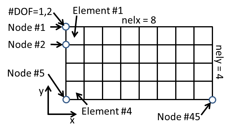
The numbering rule for elements and nodes
The template code assumes a rectangular design domain, where each element is modeled as a unit square. The numbering of elements and nodes are explained in the figure below.
Input parameters
Inputs to the program are (1) the number of elements in the x and y directions (nelx and nely),
(2) the volume fraction (volfrac, this is the number between 0 and 1 that specifies the
ratio between the volume of the target topology and the maximum volume \(nelx \times nely\)), (3) the penalty
parameter of the Young’s Modulus model (penal, usually =3), and (4) the filter radius (rmin,
usually =3).
Material properties
%% MATERIAL PROPERTIES
E0 = 1;
Emin = 1e-9;
nu = 0.3;
Set the Young’s Modulus (E0), and the Poisson’s ratio (nu). Leave Emin as a small number.
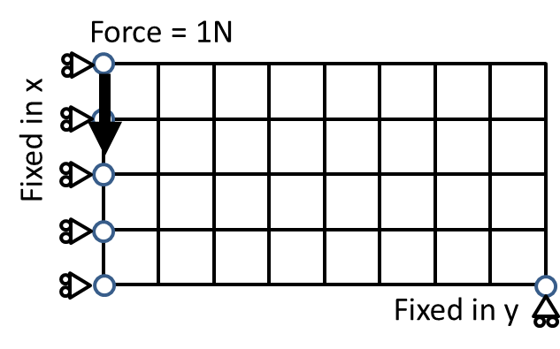
Define loadings
F = sparse(2,1,-1,2*(nely+1)*(nelx+1),1);This line specifies the loading. Here F is a sparse column vector with 2(nely+1)(nelx+1) elements.
(2,1,-1,\cdots) specifies that there is a force of -1 at the second row and first column
of the vector. According to the numbering convention of this code, this is to say that in the y direction
of the first node, there is a downward force of magnitude 1.
Define boundary conditions (Fixed DOFs)
fixeddofs = union([1:2:2*(nely+1)],[2*(nelx+1)*(nely+1)]);This line specifies the nodes with fixed DOFs. [1:2:2*(nely+1)] are x directions
of all nodes to the left side of the structure, and 2*(nelx+1)*(nely+1) is the y direction
of the last node (right bottom corner). See figure below:
Numbering of dofs, nodes, and elements in the 88 line code.
Filtering of sensitivity (gradient)
Pure gradient descent may result in a topology with checkerboard patterns. See figure below. While mathematically sound, such a solution can be infeasible from a manufacturing perspective or too expensive to realize (e.g., through additive manufacturing of porous structures). Therefore, a smoothed solution is often more preferred.
%20A%20review%20and%20generalization%20of%202-D%20structural%20topology%20optimization%20using%20material%20d.files/image226.jpg)
In the code we prepare a Gaussian filter, through the following code:
%% PREPARE FILTER
iH = ones(nelx*nely*(2*(ceil(rmin)-1)+1)^2,1);
jH = ones(size(iH));
sH = zeros(size(iH));
k = 0;
for i1 = 1:nelx
  for j1 = 1:nely
    e1 = (i1-1)*nely+j1;
    for i2 = max(i1-(ceil(rmin)-1),1):min(i1+(ceil(rmin)-1),nelx)
      for j2 = max(j1-(ceil(rmin)-1),1):min(j1+(ceil(rmin)-1),nely)
        e2 = (i2-1)*nely+j2;
        k = k+1;
        iH(k) = e1;
        jH(k) = e2;
        sH(k) = max(0,rmin-sqrt((i1-i2)^2+(j1-j2)^2));
      end
    end
  end
end
H = sparse(iH,jH,sH);
Hs = sum(H,2);
The design sensitivity can then filtered by
dc(:) = H*(x(:).*dc(:))./Hs./max(1e-3,x(:));Topology optimization with local density constraints
One drawback of the topology optimization formulation we discussed above is that the resultant topologies often have sparse structures (please test to see). In nature we observe structures that are denser and porous, e.g., bones, nests, etc, with more connecting “beams” of smaller dimensions. One of the key benefit of such structures is reliability, i.e., the failure of some beams will not drastically change the performance of the whole. Yet with sparse structures produced from our optimization, the reliability can be low.
Wu et al. recently proposed a formulation that incorporates local density constraints instead of the global volume fraction constraint. The following sample code is our implementation of Wu’s method on solving compliance problems.
%% This code follows Wu et al. (https://arxiv.org/pdf/1608.04366.pdf)
%% Augmented Lagrangian is implemented instead of MMA.

%% Input
nelx=400; % horizontal length
nely=200; % vertical length
alpha=0.6; % lobal volume fraction
alpha2=0.6; % global volume fraction
gamma=3.0; % material binarization
rmin=3.0; % filter radius
density_r = 6.0/1; % density radius

%% Algorithm parameters
p = 16;
beta=10.0;
nn = nelx*nely;
epsilon_al=1;
epsilon_opt=1e-3;

% PREPARE FILTER
% create neighbourhood index for M (filtering)
r = rmin;
range = -r:r;
[X,Y] = meshgrid(range,range);
neighbor = [X(:), Y(:)];
D = sum(neighbor.^2,2);
rn = sum(D<=r^2 & D~=0);
pattern = neighbor(D<=r^2 & D~=0,:);
[locX, locY] = meshgrid(1:nelx,1:nely);
loc = [locY(:),locX(:)];
M = zeros(nn,rn);
for i = 1:nn
    for j = 1:rn
        locc = loc(i,:) + pattern(j,:);
        if sum(locc<1)+sum(locc(1)>nely)+sum(locc(2)>nelx)==0
            M(i,j) = locc(1) + (locc(2)-1)*nely;
        else
            M(i,j) = NaN;
        end
    end
end
% M_t = M';
% idx = kron((1:nn)',ones(rn,1));
% idy = M_t(~isnan(M_t));
% idx(isnan(M_t))=[];
% bigM = sparse(idx,idy,1);
iH = ones(nelx*nely*(2*(ceil(rmin)-1)+1)^2,1);
jH = ones(size(iH));
sH = zeros(size(iH));
k = 0;
for i1 = 1:nelx
  for j1 = 1:nely
    e1 = (i1-1)*nely+j1;
    for i2 = max(i1-(ceil(rmin)-1),1):min(i1+(ceil(rmin)-1),nelx)
      for j2 = max(j1-(ceil(rmin)-1),1):min(j1+(ceil(rmin)-1),nely)
        e2 = (i2-1)*nely+j2;
        k = k+1;
        iH(k) = e1;
        jH(k) = e2;
        sH(k) = max(0,rmin-sqrt((i1-i2)^2+(j1-j2)^2));
      end
    end
  end
end
H = sparse(iH,jH,sH);
Hs = sum(H,2);
bigM = H>0;

% create neighbourhood index for N (local density)
r = density_r;
range = -r:r;
mesh = range;
[X,Y] = meshgrid(range,range);
neighbor = [X(:), Y(:)];
D = sum(neighbor.^2,2);
rn = sum(D<=r^2);
pattern = neighbor(D<=r^2,:);
[locX, locY] = meshgrid(1:nelx,1:nely);
loc = [locY(:), locX(:)];
N = zeros(nn,rn);
for i = 1:nn
    for j = 1:rn
        locc = loc(i,:) + pattern(j,:);
        if sum(locc<1)+sum(locc(1)>nely)+sum(locc(2)>nelx)==0
            N(i,j) = locc(1) + (locc(2)-1)*nely;
        else
            N(i,j) = NaN;
        end
    end
end
idx = kron((1:nn)',ones(rn,1));
N_t = N';
idy = N_t(~isnan(N_t));
idx(isnan(N_t))=[];
bigN = sparse(idx,idy,1);
N_count = sum(~isnan(N),2);

%% MATERIAL PROPERTIES
E0 = 1;
Emin = 1e-9;
nu = 0.3;

%% PREPARE FINITE ELEMENT ANALYSIS
A11 = [12  3 -6 -3;  3 12  3  0; -6  3 12 -3; -3  0 -3 12];
A12 = [-6 -3  0  3; -3 -6 -3 -6;  0 -3 -6  3;  3 -6  3 -6];
B11 = [-4  3 -2  9;  3 -4 -9  4; -2 -9 -4 -3;  9  4 -3 -4];
B12 = [ 2 -3  4 -9; -3  2  9 -2;  4  9  2  3; -9 -2  3  2];
KE = 1/(1-nu^2)/24*([A11 A12;A12' A11]+nu*[B11 B12;B12' B11]);
nodenrs = reshape(1:(1+nelx)*(1+nely),1+nely,1+nelx);
edofVec = reshape(2*nodenrs(1:end-1,1:end-1)+1,nelx*nely,1);
edofMat = repmat(edofVec,1,8)+repmat([0 1 2*nely+[2 3 0 1] -2 -1],nelx*nely,1);
iK = reshape(kron(edofMat,ones(8,1))',64*nelx*nely,1);
jK = reshape(kron(edofMat,ones(1,8))',64*nelx*nely,1);

% DEFINE LOADS AND SUPPORTS (HALF MBB-BEAM)
F = sparse((nely+1)*2*nelx+nely+2,1,-1,2*(nely+1)*(nelx+1),1);
U = zeros(2*(nely+1)*(nelx+1),1);
fixeddofs = 1:2*(nely+1);
alldofs = [1:2*(nely+1)*(nelx+1)];
freedofs = setdiff(alldofs,fixeddofs);

%prepare some stuff to reduce cost
dphi_idphi = bsxfun(@rdivide,H,sum(H));

%% START ITERATION
phi = alpha*ones(nn,1);
loop = 0;
delta = 1.0;
count=0;
count_final=1;

figure
while beta < 3000
    if mod(loop,1)==0
        step=1;
    end
    loop = loop + 1;
    loop2 = 0;
    %augmented lagrangian parameters
    r = 1;
    r2 = 0.001;
    lambda = 0;
    lambda2 = 0;
    eta = 0.1;
    eta2 = 0.1;
    epsilon = 1;
    dphi = 1e6;

    %%%%%%%%%%%%%%%%%%%%%%%%%%%%%%%%%%%%%%%%%%%%%%%%%%%%%%%%%%%%%%%%%%%%
    %%%%%%%%%% Get initial g and c %%%%%%%%%%%%%%%%%%%%%%%%%%%%%%%%%%%%%
    phi_til = H*phi(:)./Hs;
    rho = (tanh(beta/2)+tanh(beta*(phi_til-0.5)))/(2*tanh(beta/2));
    sK = reshape(KE(:)*(Emin+rho(:)'.^gamma*(E0-Emin)),64*nelx*nely,1);
    K = sparse(iK,jK,sK); K = (K+K')/2;
    U(freedofs) = K(freedofs,freedofs)\F(freedofs);
    ce = sum((U(edofMat)*KE).*U(edofMat),2);
    c = sum(sum((Emin+rho(:).^gamma*(E0-Emin)).*ce));
    rho_bar = bigN*rho./N_count;
    g = (sum(rho_bar.^p)/nely/nelx)^(1/p)/alpha - 1.0;
    global_density = rho'*ones(nn,1)/nn-alpha2;
    %%%%%%%%%%%%%%%%%%%%%%%%%%%%%%%%%%%%%%%%%%%%%%%%%%%%%%%%%%%%%%%%%%%%

    phi_old = phi;

    while 1
        if (max(abs(full(dphi)))<epsilon_al && g<0.005 && loop2>0) || (loop2 > 100)
            break;
        end
        loop2 = loop2 + 1;
        dphi = 1e6;
        j=0;j2=0;
        loop3 = 0;

        while max(abs(full(dphi))) > epsilon && loop3 < 10000
            loop3 = loop3 + 1;
            learning_rate = 0.001;

            dc_drho = -gamma*rho.^(gamma-1)*(E0-Emin).*ce(:);
            drho_dphi = beta*(1-tanh(beta*(phi(:)-0.5)).^2)/2/tanh(beta/2);
            dc_dphi = sum(bigM.*bsxfun(@times, dphi_idphi, (dc_drho.*drho_dphi)'),2);
            dg_drhobar = 1/alpha/nn*(1/nn*sum(rho_bar.^p)).^(1/p-1).*rho_bar.^(p-1);
            dg_dphi = sum(bigM.*bsxfun(@times, dphi_idphi, (bigN*(dg_drhobar./N_count).*drho_dphi)'),2);
            dphi = dc_dphi + lambda*dg_dphi*(g>0) + 2/r*g*dg_dphi*(g>0) +...
                lambda2*ones(nn,1)/nn*(global_density>0) + 2/r2*global_density/nn/nn*ones(nn,1)*(global_density>0);

            % check if learning rate is too large
            g_old = g;
            global_density_old = global_density;
            c_old = c;
            loop4 = 0;
            while loop4 < 10
                delta = -dphi*learning_rate;
                phi_temp = phi + delta;
                phi_til = H*phi_temp(:)./Hs;
                rho_temp = (tanh(beta/2)+tanh(beta*(phi_til-0.5)))/(2*tanh(beta/2));
                rho_bar_temp = bigN*rho_temp./N_count;
                g_temp = (sum(rho_bar_temp.^p)/nely/nelx)^(1/p)/alpha - 1.0;
                global_density_temp = rho_temp'*ones(nn,1)/nn-alpha2;
                sK = reshape(KE(:)*(Emin+rho_temp(:)'.^gamma*(E0-Emin)),64*nelx*nely,1);
                K = sparse(iK,jK,sK); K = (K+K')/2;
                U(freedofs) = K(freedofs,freedofs)\F(freedofs);
                ce_temp = sum((U(edofMat)*KE).*U(edofMat),2);
                c_temp = sum(sum((Emin+rho_temp(:).^gamma*(E0-Emin)).*ce_temp));
                dobj = (c_temp + lambda*g_temp*(g_temp>0) + 1/r*g_temp^2*(g_temp>0) + 1/r2*global_density_temp^2*(global_density_temp>0))-...
                    (c_old + lambda*g_old*(g_old>0) + 1/r*g_old^2*(g_old>0) + 1/r2*global_density_old^2*(global_density_old>0));
                if dobj>0
                    learning_rate = learning_rate*0.5;
                    loop4 = loop4 + 1;
                    if loop4 == 10
                        loop3 = 10000;
                        dphi = 0;
                    end
                else
                    phi = phi_temp;
                    c = c_temp;
                    g = g_temp;
                    ce = ce_temp;
                    rho = rho_temp;
                    rho_bar = rho_bar_temp;
                    global_density = global_density_temp;
                    break;
                end
            end
            %% PRINT RESULTS

            fprintf(' It.:%5i Obj.:%11.4f g:%7.3f eta:%7.3f r:%7.3f ch.:%7.3f\n',loop, c, ...
            g, eta, log(r), max(abs(full(dphi))));

            %% PLOT DENSITIES
            colormap(gray); imagesc(1-reshape(rho,[nely,nelx])); caxis([0 1]); axis equal; axis off; drawnow;

            if mod(count,2)==0
                saveas(gcf,sprintf('infill%d.png',count_final))
                count_final=count_final+1;
            end
            count=count+1;
        end

        if g<eta
            lambda = lambda + 2*g/r;
            j = j+1;
            eta = eta*0.5;
        else
            r = 0.5*r;
            j = 0;
        end

        if global_density<eta2
            lambda2 = lambda2 + 2*global_density/r2;
            j2 = j2+1;
            eta2 = eta2*0.5;
        else
            r2 = 0.5*r2;
            j2 = 0;
        end
    end

    delta = full(max(abs(phi-phi_old)));

    % step 17
    beta = 2*beta;

end