ANSYS DOE and Design Optimization Tutorial

by Max Yi Ren and Aditya Vipradas

Table of Contents

1. Introduction
2. A Running Example
   1. Description of the brake design problem
   2. Static structural setup
   3. Modal setup
   4. Transient thermal setup
   5. Transfering geometry and model across analysis modules
   6. Define input parameters
3. Background Knowledge
4. Design of Experiments
5. Sensitivity Analysis
6. Optimization
7. Checklist

Introduction

This is a step-by-step tutorial of the ANSYS Design of Experiment (DOE) and Optimization tools. These tools will allow you to better validate and understand your engineering model and further refine your design for specific properties of interest. We will skip some mathematical details but focus on explaining how things should be done.

We encourage you to also read related chapters in the official ANSYS Design Exploration User’s Guide.

NOTE: This tutorial is tested on ANSYS 16, 17.1 and 17.2.

A Running Example

Before we start, please prepare the CAD model of your design and determine attributes that you want to design for. You can also use the following sample problem on vehicle brake design. The model file of the brake can be downloaded here (.agdb). The raw model is here (.stp). All credits go to A. Durgude, A. Vipradas, S. Kishore, and S. Nimse (see their MAE598 Design Optimization project report (2016)).

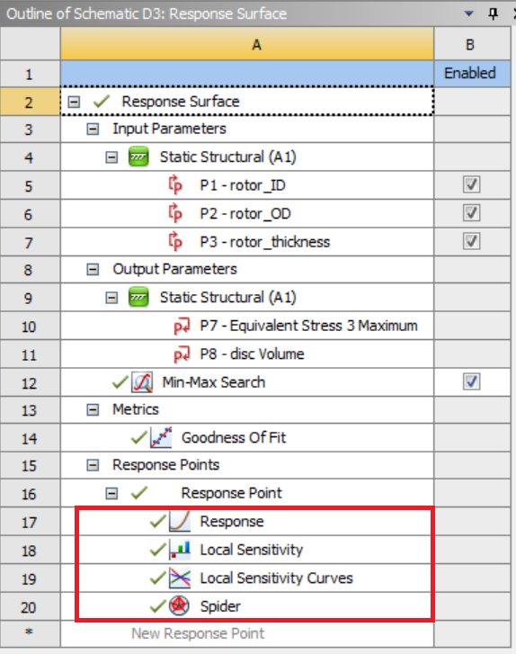
Description of the brake design problem

To summarize, the brake design problem has the following objectives:

• Design a brake disc for emergency braking conditions with minimal volume
• Minimize the maximum stress in the brake disc
• Maximize the first natural frequency of the brake disc
• Minimize the maximum temperature in the brake disc

The three subsystems are as follows:

• Structural Analysis: The brake disc has to sustain the pressure from the hydraulically actuated brake pads during sudden braking conditions. Stresses are induced due to friction between the brake pads and the disc. The disc also experiences centrifugal body forces due to its rotation. Resultant stresses generated due these forces can lead to material failure. Therefore, it is of prime importance to make sure that the stresses in the disc are minimized.

• Modal Analysis: Free modal analysis is performed to ensure that the disc’s first natural frequency is higher than the engine firing frequency. This guarantees that the disc does not experience failure due to resonance.

• Thermal Analysis: Braking in a vehicle takes place due to friction between the brake pads and the rotor disc. This leads to heat flux generation in the disc which consequently results in increase in its temperature and thermal stresses. Emergency braking conditions induce high temperatures that damage the contact surfaces. It is therefore essential to minimize the temperature to prevent disc wear and tear.

The following sections describes how these analysis are set up.

Static structural setup

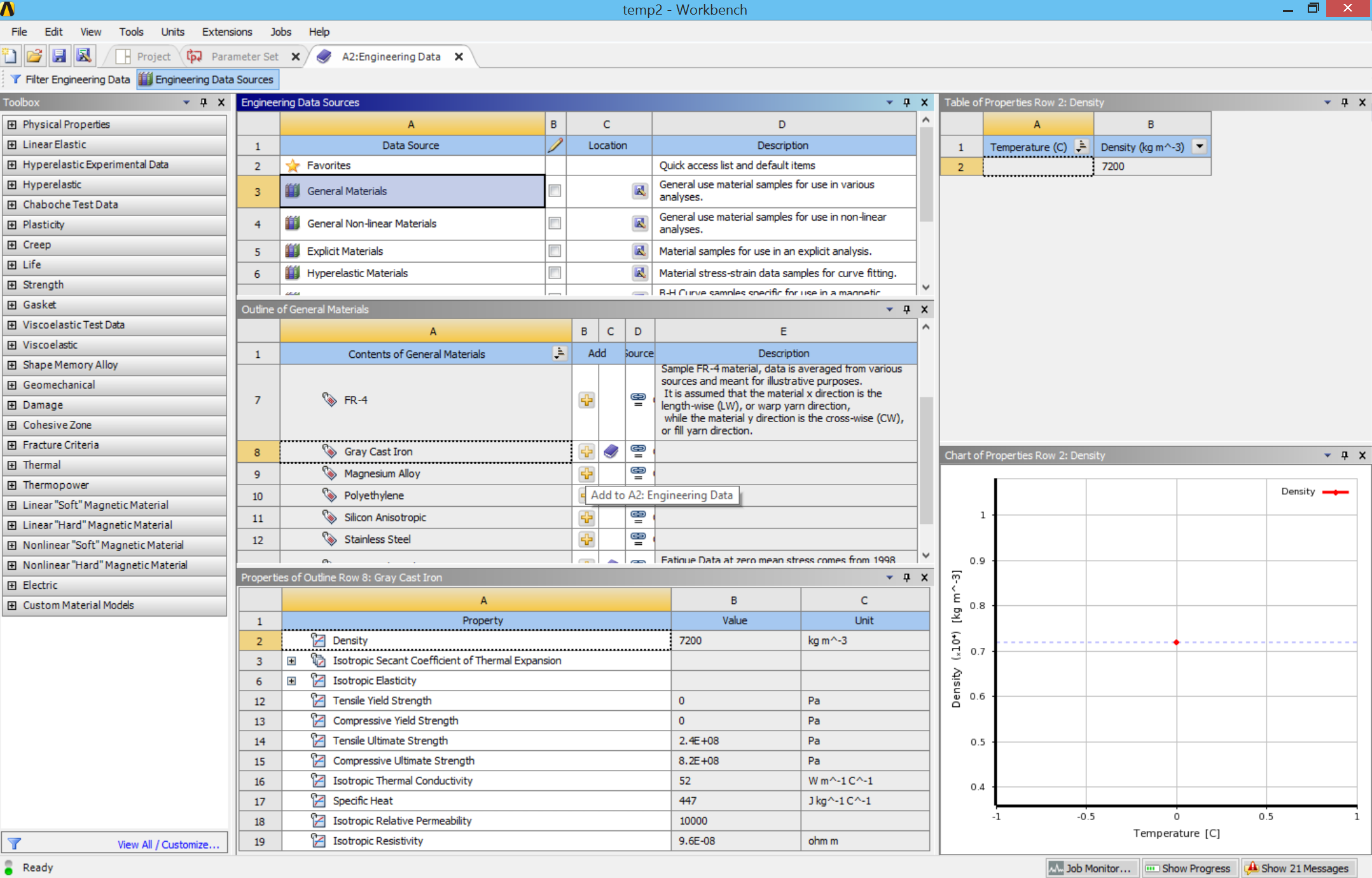
• Define Material: In Project Schematic, click on Engineering Data, then click Engineering Data Sources->General Materials, from the list, find “Gray Cast Iron” and click the “add” button (the plus sign). The sign with a blue book will appear after we assign this material to an object.

• Load Geometry: In Project Schematic, click on Geometry, then create geometry in DesignModeler or import a agdb file.

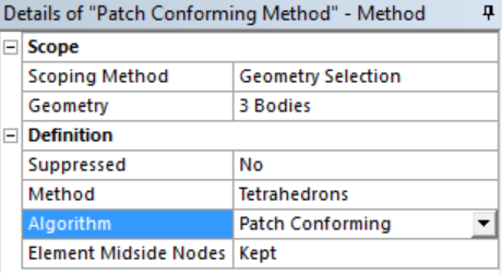
• Mesh the Geometry: In Project Schematic, double click on Model to open the Mechanical screen. To setup the mesh: Right click Mesh -> Method -> Select all the bodies and then select Tetrahedrons in Method option

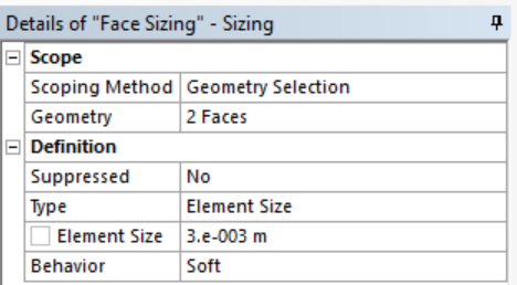
• Right click Mesh -> Sizing -> Select inner faces of the brake pads and set element size to 3 mm. This is because the pad is relatively thin, and has higher stress concentration than other places. Therefore finer mesh will give us more accurate simulation result. NOTE: For student version, you may not be able to run the simulation if the mesh size is higher than the limitation.

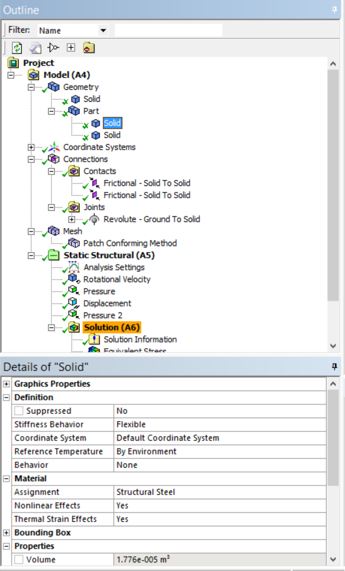
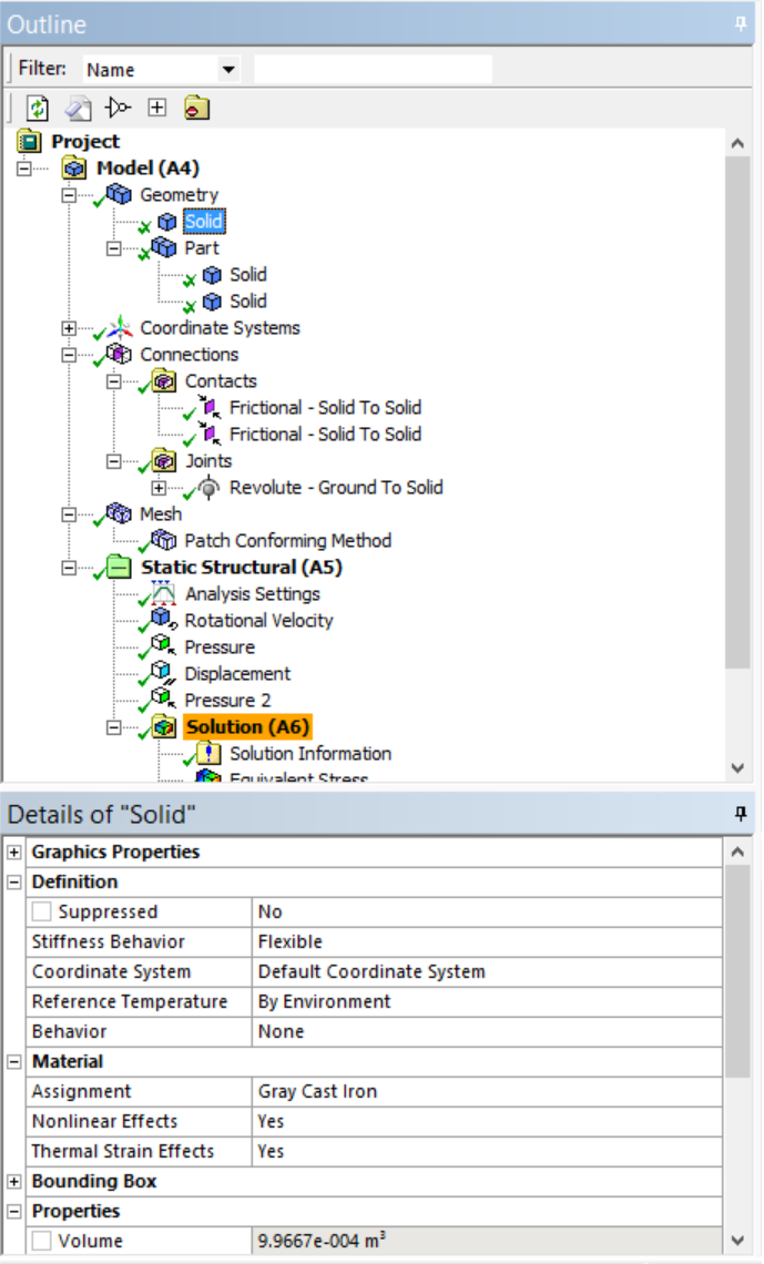
• Assign Material: Still in the Mechanical screen, notice the two parts under Geometry in the outline window. These are the brake disk and the brake pads. Assign material types by clicking on each, and go to the Details window below the outline, find Material->Assignment, choose Gray Cast Iron for the disk, and Structural Steel for the pads.

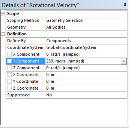
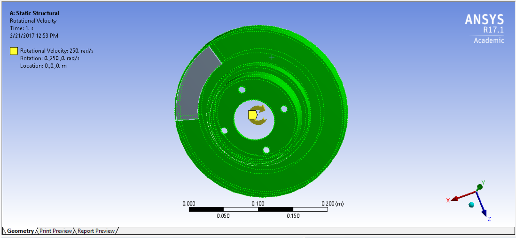
• Define Boundary Conditions: Right click Static Structural -> Insert -> Rotational Velocity -> Set 250 rad/s to the y-axis of the brake disk.

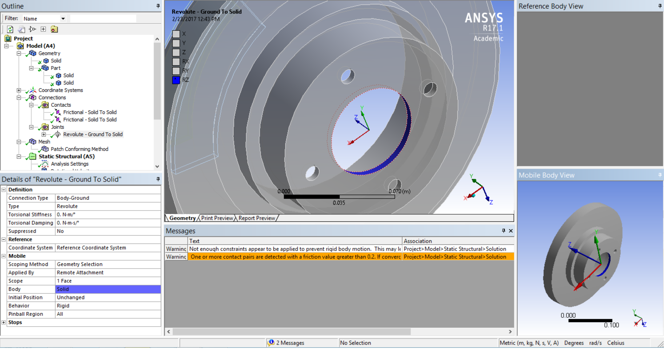
• Right click on Connections, create a Revolute Joint. Set up the joint as shown below: In Details, choose “Body-Ground” for “connection type”, choose the highlighted (blue) circle for “scope”.

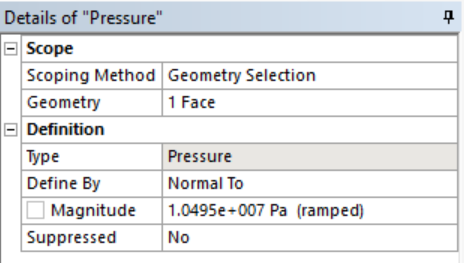
• Right click Static Structural -> Insert -> Pressure -> Enter the values as shown by selecting the outer brake pad faces. Do this for each outer brake pad face.

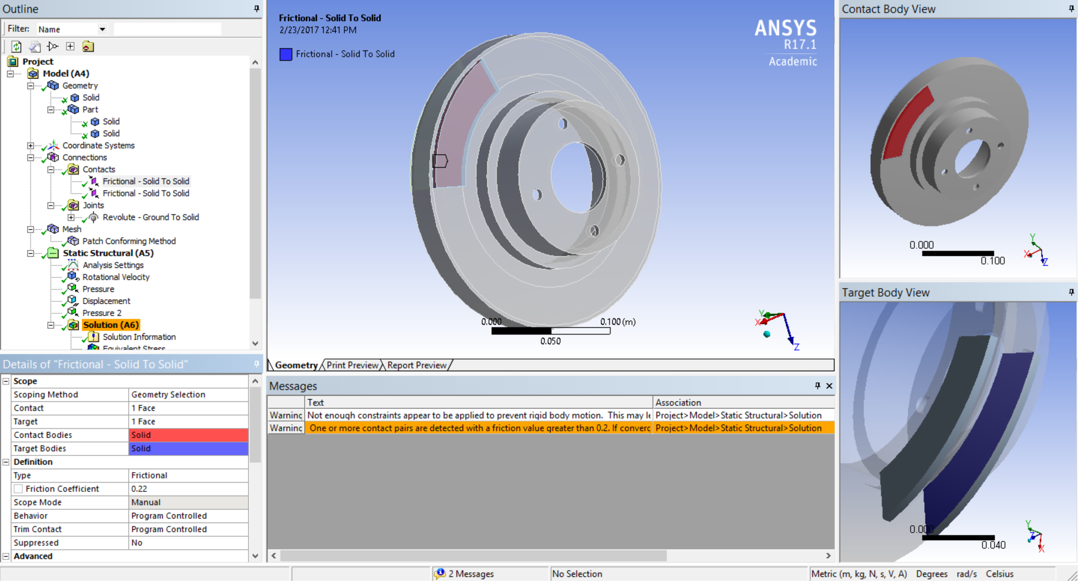
• Click on Connections->Contacts in the outline window, and right click to add Manual Contact Region. Set up a frictional contact as shown below. Do this for both contact regions between the pads and the disk.

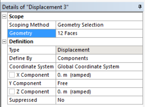
• Right click Static Structural -> Insert -> Displacement -> Fix x- and z-axis displacement of all the faces of brake pads

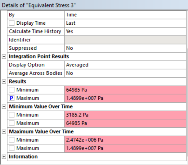
• Select the desired output values and solve by right clicking on Solution and hitting Solve. Set Equivalent von-Mises stress as output parameter.

• Note that the solution is sensitive to various settings, including mesh size, nonlinear and thermal strain effects of the chosen materials, and whether large deflection is considered.

Modal setup

• Drag Modal Analysis box on the Geometry of Static Structural box. Same geometry and mesh settings as discussed earlier.
• Right click Brake pad parts in Geometry -> Click Suppress (We want the natural frequency of the brake disc only)
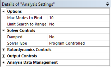
• Click Analysis Settings and enter “Max Modes to Find” as 10

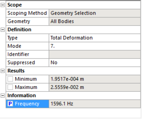
• Right click Solution -> Insert -> Deformation -> Total -> Enter the desired mode number. The first 6 modes are the rigid body modes. We do not need those. Parametrize the frequency of mode 7 which is the first deformation mode.

Transient thermal setup

• Drag Transient Thermal box on the Geometry tab of the Static Structural box.
• Same Geometry and Mesh settings as Static Structural. Suppress brake pad geometry as explained in the Modal module.
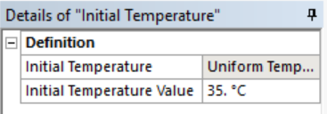
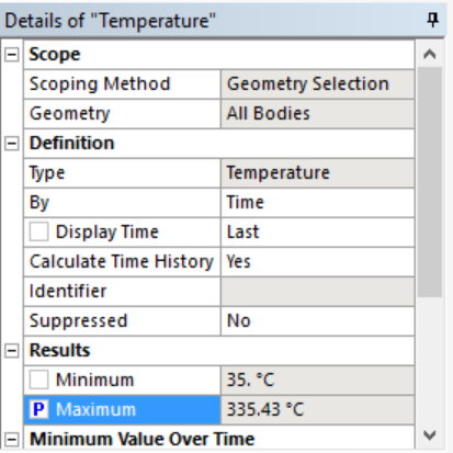
• Under Transient Thermal click “Initial Temperature” and set the value to 35C.

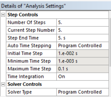
• Click on “Analysis Settings” and set up the values as shown.

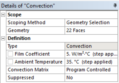
• Right click Transient Thermal -> Insert -> Convection -> Select all the brake disc faces and set the values as shown.

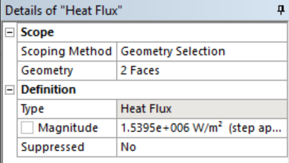
• Right click Transient Thermal -> Insert -> Heat flux -> Select the face as shown and enter the values

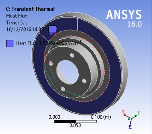
• Repeat this for the faces on the other side of the brake disc

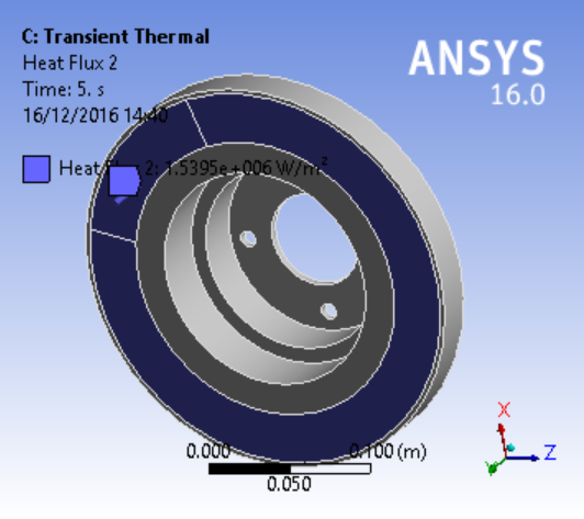
• Right click Solution -> Insert -> Thermal -> Temperature, parameterize and solve

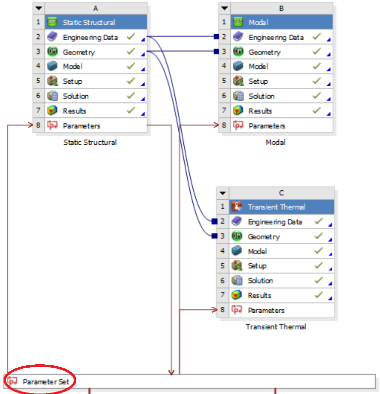
Transfering geometry and model across analysis modules

Consider that you have performed a Static Structural Analysis, you can use the mesh created from this analysis to perform another analysis, say a modal analysis. The followings steps show how this is done.

1. To copy the geometry to another analysis

2. Hold on the Modal module

1. Drag onto the tab of the Static Structural Module

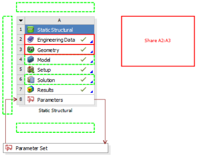
1. The geometry is shared

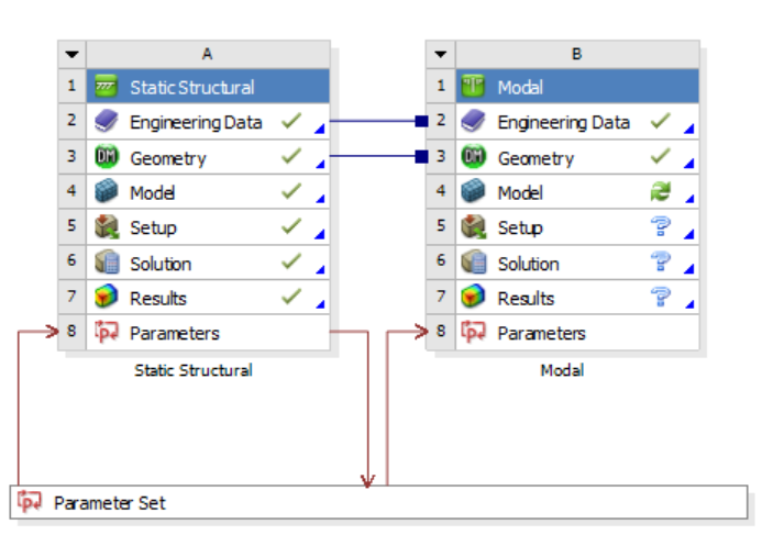
This is generally performed when two different analyses are to be performed on the same geometry. You will have to do the mesh again.

1. To share the mesh, boundary conditions setup and results

2. Hold on the Modal module

3. Drag on the Model or Solution tab of the Static Structural module

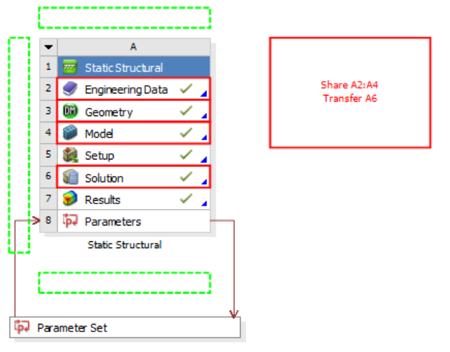
1. The mesh, setup and results are shared

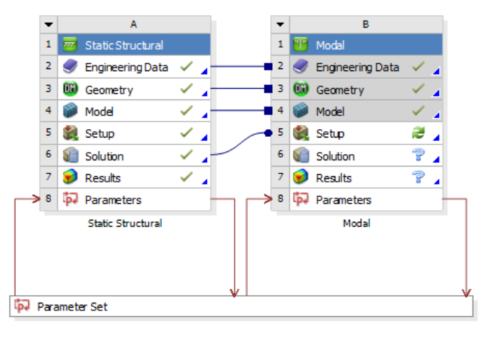
This is generally performed when results from one analysis are to be shared with another analysis. For instance, these steps can be used to perform pre-stressed modal analysis where results from static structural analysis are shared with modal analysis.

NOTE: You have only these two options. There is no option to just share the mesh.

Define input parameters

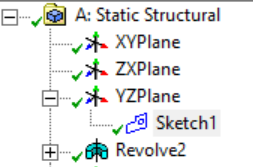
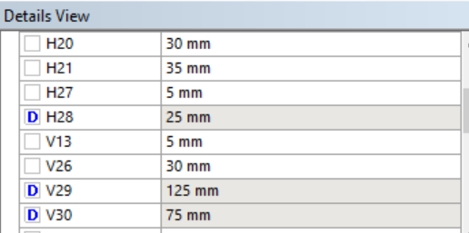
The input parameters are the design variables. To set these up, click on the Geometry tab of the static structural box. Parametrize the outer diameter, inner diameter and thickness of the brake disc. Click on Sketch 1 as shown.

Select the dimensions as input parameters as shown in the figure by hitting the checkbox.

Background Knowledge for DOE and Optimization

We first need to define some terminologies for a design problem:

• Parameters: These include all available “nobs” for your design, e.g., geometry, topology, materials, and control gains.
• Variables: These are the subset of design parameters that you want to tune (so the rest of the parameters are fixed during the design). The set of all possible variable settings is called the design space.
• Objectives: An objective defines the goodness of a design. This is usually some performance of the design that you care about (safety of a car, stability of a controller, etc.). In many cases, we are interested in designing for more than one objective. However, to make things easier, our discussion will be focused on a single objective. We will talked about how multiple objectives can be handled.
• Constraints: These are functions of the design variables that define a feasible variable space. E.g., the design of a bridge has to have a maximum stress less than the critical stress (times a safety factor).

NOTE: In ANSYS and some other software, the difference between parameters and variables is not distinguished. So when you see “parameters”, it might actually mean “variables”.

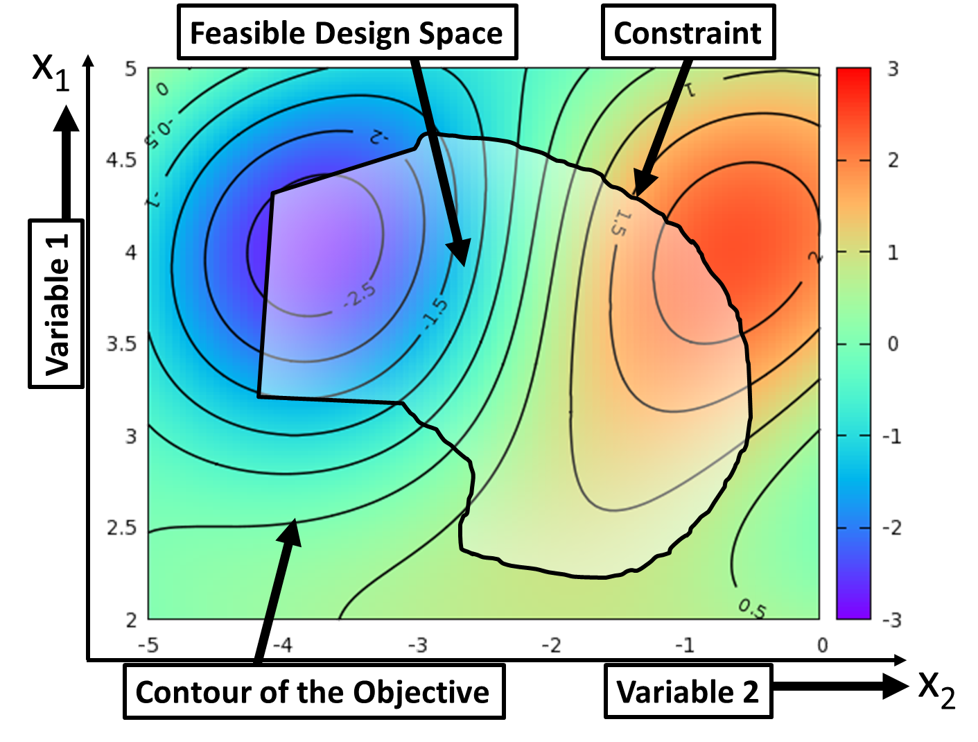
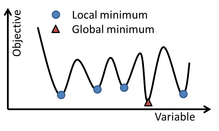
Optimization is the iterative process for finding a design that maximizes or minimizes the objective by searching the design space. There are two major schools of optimization algorithms: gradient-based methods are useful when the objective is differentiable (in many mathematical and machine learning problems). They are fast but can only find local solutions; Gradient-free methods are useful when the evaluation of the objective (and its gradient) is expensive or when the gradient is noisy. Ansys offers both options.

DOE: Many engineering design problems have objectives that are evaluated through expensive simulations/experiments, e.g., CFD analysis. In such cases, each function evaluation during the optimization takes a long time, and thus could making the optimization intractable. DOE is a set of methodologies that determine which design to evaluate from a potentially large design space, so that we can create a statistical model to predict the objective values of other designs with low uncertainty in prediction. Through the predictive model, we can also tell the sensitivity of variables, i.e., whether the objective changes much with respect to each of the variables. DOE is often used as part of the gradient-free optimization algorithm.

Design of Experiments

DOE is used to effectively sample a design space (e.g., all design parameters for the brake disc) so that a statistical model can be built to predict responses (e.g., the maximum stress, or the first natural frequency, or the maximum temperature) of a given design. DOE is useful when one can only sample a limited number of points (i.e., run a limited number of simulations). The key idea of DOE is to ``spread out’’ the samples so that the resultant statistical model has low uncertainty in its model estimation and thus high accuracy in prediction.

Step 1: Define parameters and responses

To conduct DOE for a given model, we shall first define the list of design variables and objectives that we care about (In Ansys, these are called input and output parameters). To do so, open the “Project Schematic” window, which shall look like this:

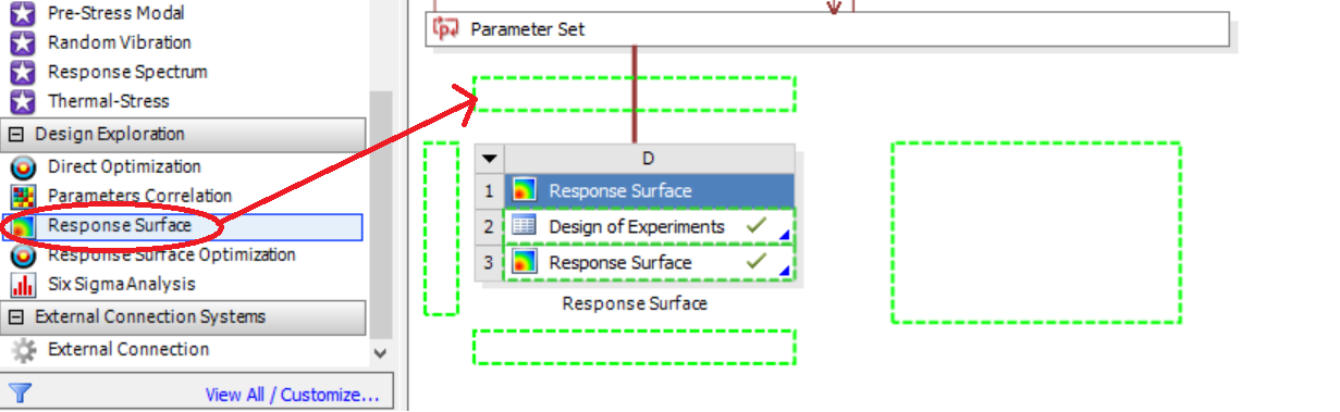
Step 2: Choose a Design Exploration method

In the Design Exploration window, find “Response Surface”. This will allow us to perform DOE for the purpose of creating a predictive model, called a response surface. Drag the “Response Surface” tab from the Toolbox on any one dashed box near “Parameter Set”.

Step 3: Choose a DOE method

While ANSYS provides various DOE methods, we suggest Latin Hypercube Sampling (LHS) and Optimal space filling with user defined sample points. The main advantage of these methods is that the number of samples is independent from the number of parameters. Another (more advanced) choice is sparse grid, which only samples a few points initially and adaptively add new sample points based on the response surface. Kriging with auto-refinement has a similar effect. Note, we do not recommend Central Composite Design (CCD) because in many cases, the objective cannot be approximated as a quadratic function, and CCD requires a large number of samples for relatively small number of variables.

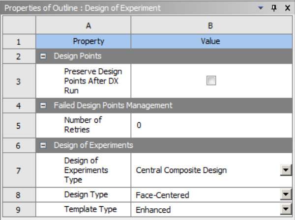
Click on the “Design of Experiments” option and select the required DOE and Design type:

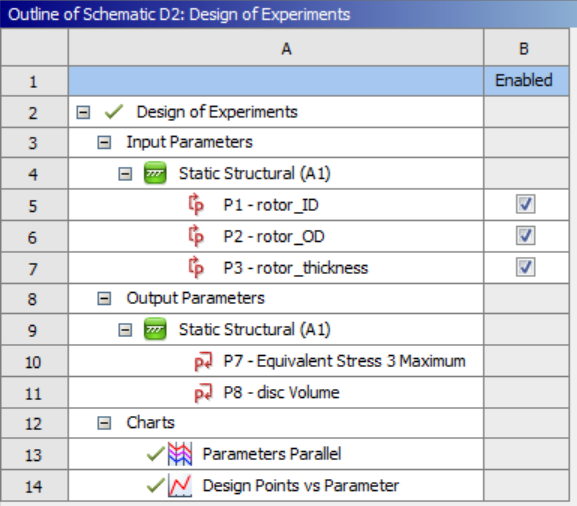
If you double click on the “Design of Experiments” tab, a new window opens where you see your input and output parameters.

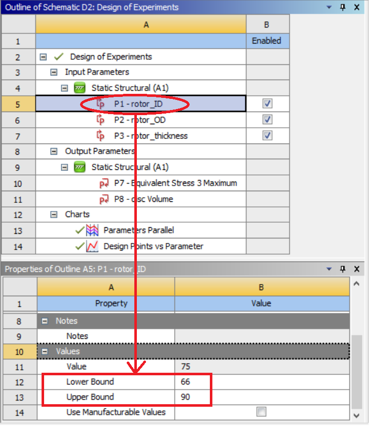
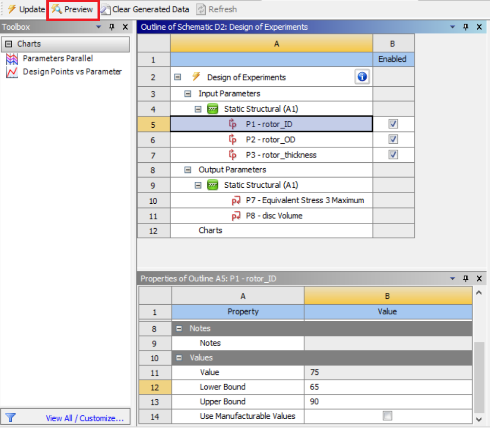
You can set the lower and upper bounds of each input parameter by clicking on that parameter.

After setting the input parameter bounds, hit “Preview” to see the list of DOE points according to your settings.

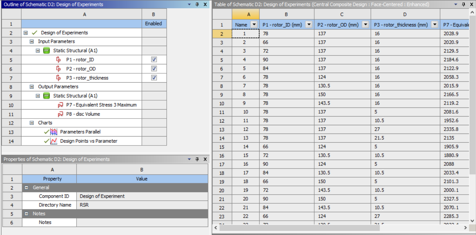
Now hit “update” and brew your coffee. Depending on how many samples you requested, it will take hours to days for DOE to finish.

NOTE: Some of your DOE samples may not be evaluated successfully due to significant change in geometry. In the brake disk example, if the outer radius of the disk is changed to be smaller than the outer radius of the pads, the friction contact setting will need to be reset manually due to mesh change. When this happens, it could indicate that some of the designs sampled by DOE are not meaningful, e.g., having the brake pads partially cover the disk is not a good design after all. It could also happen that you do want to evaluate these designs. To do so, first manually fix issues due to parameter changes, and run the simulation(s) manually. You can then download the current DOE results, add in these manually derived data, and upload the data table to ANSYS.

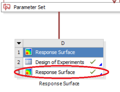
Step 4: Create a response surface

The DOE results can be used to create a response surface for prediction purpose. ANSYS provides the following list of response surface methods:

• Standard Response Surface: This method uses a polynomial surface to fit the data. It requires the least amount of computation in both fitting and prediction. However, the performance of the prediction largely depend on the choice of the polynomial bases. Use this method when you have lots of data and the change in objective is smooth.
• Kriging: This method is non-parametric, meaning that the prediction will depend on all existing data points. Thus the method could be slow in prediction when you have a large amount data to fit. It is also slow in fitting the data due to the calculation of pair-wise distances among data points. However, this method automatically fits through all data points. Use this method when your data is highly nonlinear and limited, and you want your model to fit right through your data (i.e., you trust your simulation results).
• Non-parametric Regression: This method uses Support Vector Regression. It is similar to Kriging in that the prediction depends on current data. But instead of using all data, this method chooses the most important data points to perform prediction. Thus its computation cost for prediction is less than that of Kriging. Yet, its cost of fitting is still high. The model does not fit through the data. Use this method when your data is highly nonlinear, and you don’t need your model to fit right through your data.
• Neural Network: Feedforward neural network creates a nonlinear mapping from the input (a design) to the output (its objective value) that mimics the expensive simulation. It is slow in training (and may end up with a different model each time you train, even if the data is the same) when the network is deep, but the prediction only involves simple matrix calculation and is fast. Use this method when your data is highly nonlinear but you have lots of them, and you don’t need your model to fit right through your data.
• Sparse Grid: This method goes with the corresponding DOE method. It is similar to Kriging in that it handles highly non-linear objectives. It does so by adaptively sampling in the most uncertain areas of the design space, and thus may reduce the number of samples needed. Use this method when the objective is highly nonlinear and you cannot afford many simulations

To create a response surface, click on the “Response Surface” option in the Project Schematic window:

A new window opens. Choose the type of response surface you need. And then hit on the “Update” button.

Common issues in DOE and response surface

My model has a bad fit, what shall I do?: There are two ways to improve the goodness of fit: (1) increase the sample size in DOE; and (2) increase the “complexity” of the response surface. To perform the latter, one can simply choose a high-order polynomial model or a non-parametric model such as Kriging and Non-parametric Regression.

Wow, now my model has a perfect fit, is that good?: The short answer is NO. While increasing the “complexity” lowers the “training error”, i.e., the error between the model and the data used to train the model, it is not recommended to use this method to push the goodness of fit to the limit. In fact, with non-parametric models, it is always possible to perfectly fit through all data points (one can always connect all dots manually). But by doing this, we may very likely overfit the model, so that it actually has worse prediction performance than a model with higher training error. To summarize the theory behind this, A model has better prediction performance when: the training error is low, and the model complexity is also low. Note that this is essentially what Occam’s Razor says.

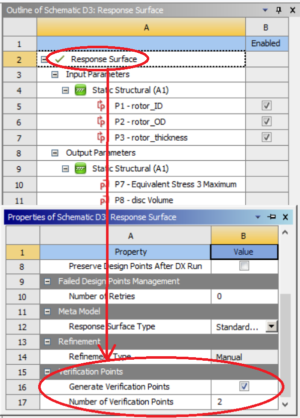
So how can we determine which model is the best? A common practice is to use a judge, or called verification points. The idea is to set some data we collected aside, and never use them for training the model, but only use them for calculating the error, which is called the validation error. The rationale is that if the model can fit well with these data without using them for training, then it has good predictability.

To perform verification in Ansys, click on the “Response Surface” as shown in the figure below. Check “Generate Verification Points” and enter the number of verification points. There is not really a rule on how many verification points you should use, but 1/4 or 1/3 of your total sample size is practically reasonable.

What if my verification result is bad? This can commonly happen if (1) your sample size is small, or (2) the underlying response is highly nonlinear, or (3) the choice of response surface is too flexible (e.g., Kriging), thus causing overfit. To address this issue, you can (1) increase the sample size, (2) try a different model. Note that in ANSYS, you can include the verfication points as refinement points, which will lead to better goodness of fit. To do so, right click on the verification point. One shall then increase the number of verification points in the response surface setting before updating the response surface (or otherwise all points are used for fitting the response surface, leading to overfitting again).

When shall I stop refinement? If the goal of creating the response surface is solely to use the surface for predicting responses, then one shall make sure that with enough verification points, the error in prediction is limited. ANSYS provides a three-star rating on the goodness of fit of the response surface for verification points for this purpose.

If the goal is to perform optimization, an accurate response surface is not necessary. Therefore with a relatively accurate surface model, one can move on to the optimization. Since the optimization is performed based on the response surface rather than the true simulations, a discrepancy may exist between the predicted and the true responses. ANSYS reports both numbers for the set of near-optimal solutions it finds. If the discrepancy is significant, one shall set these solutions as refinement points of the response surface, and run optimization again upon the refined surface. A smarter approach is the Bayesian Optimization algorithm. For interested readers, see this review of BO.

** What is verification and validation?**: “Validation” is often referred to as testing a design in reality (with experiments) while “verification” means testing the design with simulations.

Sensitivity Analysis

Building the response surface also allows us to perform sensitivity analysis, i.e., to see how much the objective changes when each variable changes. When a large number of variables exist, sensitivity analysis allows us to figure out the most important variables to design for, and thus reduce the computational cost of the optimization.

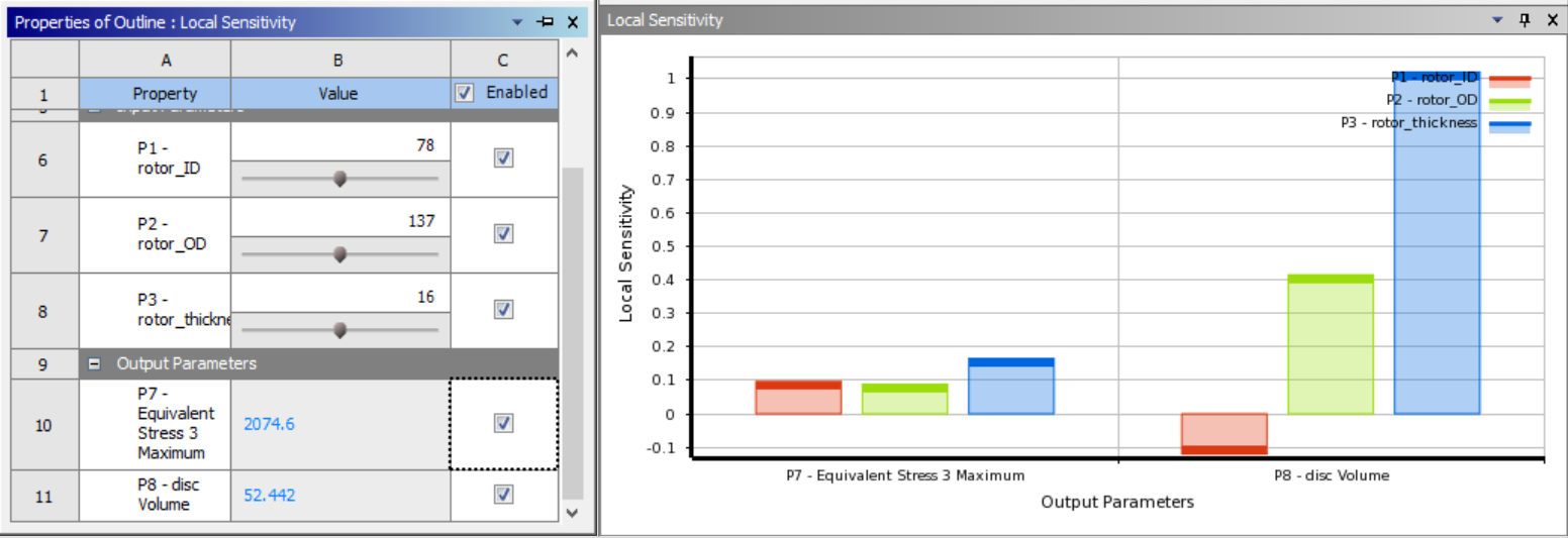
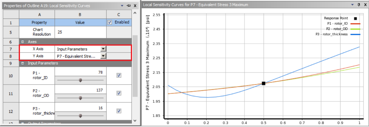
To perform sensitivity analysis, go to the “Response Surface” tab. The options for the sensitivity analysis are as shown in the figure below.

Here, “Local Sensitivity” shows the norm of the partial derivatives of the chosen objective with respect to the selected variables:

“Local Sensitivity Curves” shows the response curve of the chosen objective (Y-axis) with respect to the selected variables (X-axis):

Optimization

Single-objective vs. Multi-objective

There is rarely a design case where we only want to optimize a single response. In the running example, a set of objectives are listed. However, finding a Utopian design that simultaneously optimizes all objectives is unachievable in reality. This is because for a reasonable problem setting, there always exist conflicts among objectives. There are two solutions to this: (1) One can set one of the objectives as the objective in ANSYS, and the rest as constraints. By changing the constraints, one can derive a sequence of optimal solutions. This set of solutions is call Pareto Optimal, and a surface spanned in the space of objectives fitting through these solutions is call the Pareto frontier. For cases with two (three) objectives, it is called the Pareto curve (Pareto surface). Deriving the Pareto frontier is often more valuable than obtaining a single optimal solution, since the former reveals quantitatively how conflicting objectives trade off for the design problem of interest. % need a figure here.

Optimization algorithms

ANSYS provides a list of optimization algorithms:

• Screening: Randomly sampling the space and pick out the good ones. Use this as an initial trial to make sure everything is setup correctly, e.g., does your simulation give reasonable results?
• Multiobjective Genetic Algorithm (MOGA): Simultaneously find Pareto-optimal designs. Use this when you have multiple objectives. This is not the only choice for this situation though, see discussion above.
• Nonlinear Programming by Quadratic Lagrangian (NLPQL): Fast local search. Use this when (1) there is only one objective (but you can set other objectives as constraints), (2) the simulation does not take too long (in minutes), (3) the number of variables is small (less than 10).
• Mixed-Integer Sequential Quadratic Programming (MISQP): Similar to NLPQL, but allows integer variables. Note that the addition of integer variables will often significantly increase the computation time.
• Adaptive Single-Objective Optimization (ASO): This method uses Optimal Space Filling for DOE, Kriging as a response surface, and MISQP for finding local optimal solutions from the response surface. Use this when the evaluation of objective/constriants are expensive and you have limited budget/time for optimization.
• Adaptive Multi-Objective Optimization (AMO): Similar to ASO, this one uses Kriging and MOGA.

Things to check during your analysis and optimization

• What are your design variables, constraints, and objectives?

• What are the potential trade-offs between your objectives?

• Are your variables continuous? Or are they discrete/integer?

• Do you have analytical objective/constraint functions? And are they differentiable?

• Based on the above answers, what optimization methods will you choose?

• Perform a sensitivity analysis and comment on the importance of your variables? Also, do you observe monotonicity (i.e., the objective always goes up or down with a variable)?

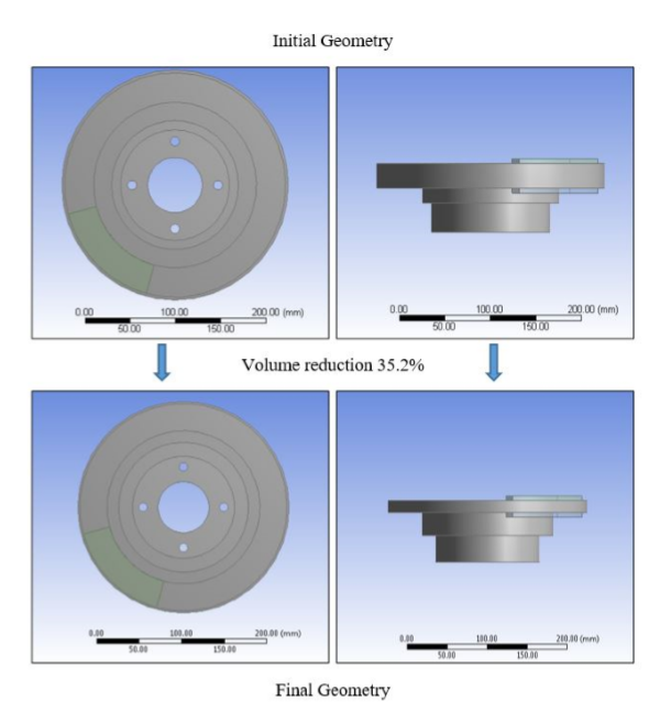
• Compare your optimal design against the initial one (e.g., see the following comparison on the brake disc design) AND comment on whether the optimal design is reasonable.